Lecture notes — Convnets
ver. 1.1.0, convnets
ver. 1.1.0 · 2026-09-02 08:24:31
Where this fits
The previous unit, Training Models, assembled a complete supervised pipeline: a loss derived as a negative log-likelihood, minibatch stochastic gradient descent with momentum or Adam, backpropagation, He initialization, and a family of explicit and implicit regularizers. All of it applies unchanged here. What changes is the model family.
A fully connected network applied to images fails on three counts, stated in the opening of Chapter 10. First, images are high dimensional: a \(224 \times 224\) RGB image is \(150{,}528\) input dimensions, and since hidden layers in fully connected networks are generally larger than the input, even a shallow network’s weight count would exceed \(150{,}528^2\), or 22 billion. Second, nearby pixels are statistically related, but a fully connected layer treats every pair of inputs equally; if the pixels of the training and test images were randomly permuted in the same way, the network could still be trained with no practical difference. Third, the interpretation of an image is stable under geometric transformations, yet shifting an image leftwards by a few pixels changes every input, so a fully connected model must learn the patterns that signify a tree separately at every position.
This unit replaces the architecture with convolutional layers, and then supplies the two mechanisms — residual connections and batch normalization — that make deep convolutional stacks trainable.
Learning outcomes
motivate-convolution— Explain why fully connected layers fail on images, and state the invariance and equivariance a convolution buys.define-1d-convolution— Define the 1D convolution operation with a shared kernel and compute its output.set-convolution-hyperparameters— Choose kernel size, stride, padding, and dilation, and predict the resulting output size.build-conv-layers-and-channels— Build a convolutional layer with multiple channels and count its parameters.reason-about-receptive-fields— Trace the receptive field of a unit through a stack of convolutional layers.extend-to-2d— Extend convolution to 2D images and read a standard image classification network.change-resolution-and-channels— Change spatial resolution and channel depth with pooling, upsampling, and 1x1 convolutions.map-vision-tasks-to-architectures— Match classification, object detection, and semantic segmentation to the architecture each needs.diagnose-deep-network-training— Explain why stacking more layers eventually makes training worse, not better.build-residual-blocks— Build a residual block and explain how skip connections restore gradient flow.apply-batch-normalization— Apply batch normalization and state what it fixes and what it costs.compare-residual-architectures— Compare ResNet, DenseNet, and U-Net as different uses of the same skip principle.explain-residual-success— Explain why residual networks work, beyond the claim that they are deeper.
Concepts introduced
- Convolutional neural network — a network predominantly composed of convolutional layers, which compute local weighted sums with parameters shared across spatial positions.
- Invariance and equivariance — \(f[t[x]] = f[x]\) and \(f[t[x]] = t[f[x]]\), the two ways a function’s output can respond to a transformed input.
- Convolution kernel — the set of trainable weights applied to each local region of the input.
- Padding — the treatment of positions where the kernel extends past the input boundary.
- Stride — the step by which the kernel advances between evaluations.
- Dilated convolution — a kernel with zeros interspersed between its weights, covering a wider region with the same weight count.
- Channels and feature maps — the parallel sets of hidden units produced by applying several kernels to the same input.
- Receptive field — the region of the original input that feeds into a given hidden unit.
- Downsampling and pooling — sub-sampling, max pooling and mean pooling, which reduce spatial resolution.
- Upsampling and transposed convolution — duplication, max unpooling, bilinear interpolation and transposed convolution, which increase spatial resolution.
- 1×1 convolution — a kernel of size one, which recombines channels at each spatial position without pooling.
- AlexNet — the eight-hidden-layer convolutional network that first performed well on ImageNet.
- VGG network — a nineteen-hidden-layer network built from small \(3 \times 3\) kernels and max pooling.
- YOLO — a single-pass object detector predicting boxes and classes over a fixed spatial grid.
- Encoder–decoder (hourglass) network — a network that downsamples to integrate context and upsamples to restore resolution.
- Sequential processing — the standard arrangement in which each layer’s output is the next layer’s only input.
- Shattered gradients — the loss of autocorrelation in the gradient with depth, which makes the loss surface unpredictable at a finite step size.
- Residual connections — branches that add a layer’s input back to its output.
- Pre-activation residual block — a block ordered activation-then-linear, so its output may be negative as well as positive.
- Bottleneck residual block — a \(1 \times 1\), \(3 \times 3\), \(1 \times 1\) sequence that reduces and then restores channel count.
- Batch normalization — standardization of each activation by batch statistics, followed by a learned scale and offset.
- Alternative normalization schemes — LayerNorm, GroupNorm, InstanceNorm and Ghost BatchNorm, which compute statistics over other axes.
- DenseNet — an architecture in which each layer receives the concatenated outputs of all preceding layers.
- U-Net — an encoder–decoder network whose encoder representations are concatenated to the decoder at matching scales.
- Stacked hourglass network — a chain of encoder–decoder blocks with additive skip links, used for pose estimation.
Invariance and equivariance
The claim that the interpretation of an image is stable under geometric transformation can be made exact. A function \(\mathbf{f}[\mathbf{x}]\) of an image \(\mathbf{x}\) is invariant to a transformation \(\mathbf{t}[\mathbf{x}]\) if
\[\mathbf{f}\big[\mathbf{t}[\mathbf{x}]\big] = \mathbf{f}[\mathbf{x}],\]
so the output is the same regardless of the transformation. A function is equivariant, or covariant, to \(\mathbf{t}[\mathbf{x}]\) if
\[\mathbf{f}\big[\mathbf{t}[\mathbf{x}]\big] = \mathbf{t}\big[\mathbf{f}[\mathbf{x}]\big],\]
so the output changes in the same way under the transformation as the input does.
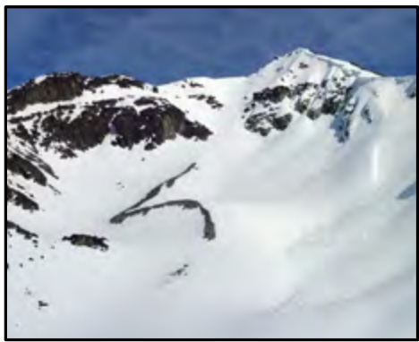
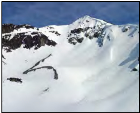
The two properties belong to different tasks. A network for image classification should be invariant to geometric transformations of the image: it should identify an image as containing the same object even if that image has been translated, rotated, flipped, or warped. Both photographs below are to be categorized as “mountain” regardless of the horizontal shift between them.
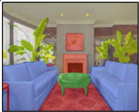
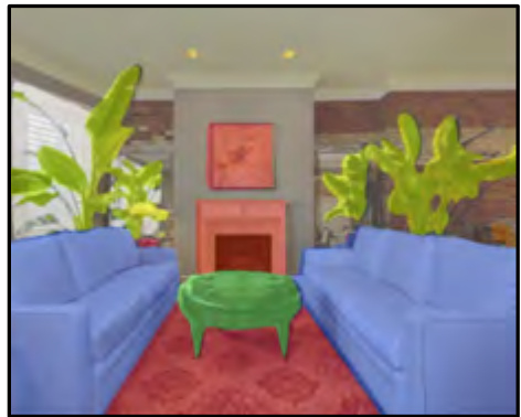
A network for per-pixel image segmentation should instead be equivariant: if the image is translated, rotated, or flipped, the network should return a segmentation that has been transformed in the same way. The coloured overlay assigns a label to each pixel, and translating the input must translate the overlay with it.
The distinction is a property of the architecture, not of the trained weights. Convolutional networks consist of a series of convolutional layers, each of which is equivariant to translation, and they typically also include pooling mechanisms that induce partial invariance to translation. The symmetry is therefore built in rather than estimated from data — which is what makes it an inductive bias rather than a learned regularity.
“Covariant” and “equivariant” are used interchangeably in Chapter 10. Neither implies invariance: an equivariant function’s output moves, an invariant function’s output does not.
A translation-equivariant layer stacked on a translation-equivariant layer is still only equivariant. Invariance for a classifier is produced by the pooling operations placed on top, and only partially. A convolutional classifier is not exactly invariant to translation.
Learning outcomes
- motivate-convolution Explain why fully connected layers fail on images, and state the invariance and equivariance a convolution buys.
Concepts
- invariance-and-equivariance invariance holds when a transformed input gives the same output, equivariance when the output undergoes the same transformation; classification wants the first, per-pixel segmentation the second
The convolution operation
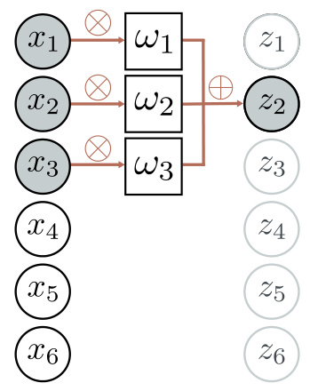
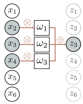
Convolutional layers are network layers based on the convolution operation. In 1D, a convolution transforms an input vector \(\mathbf{x}\) into an output vector \(\mathbf{z}\) so that each output \(z_i\) is a weighted sum of nearby inputs. The same weights are used at every position and are collectively called the convolution kernel or filter. The size of the region over which inputs are combined is the kernel size. For a kernel size of three,
\[z_i = \omega_1 x_{i-1} + \omega_2 x_i + \omega_3 x_{i+1},\]
where \(\boldsymbol{\omega} = [\omega_1, \omega_2, \omega_3]^T\) is the kernel. Translating the input translates the output in the same way, so the operation is equivariant with respect to translation.
Strictly, this is a cross-correlation and not a convolution, in which the weights would be flipped relative to the input, so \(x_{i-1}\) and \(x_{i+1}\) would be switched. The incorrect definition is the usual convention in machine learning.
Padding
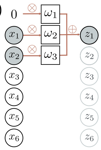
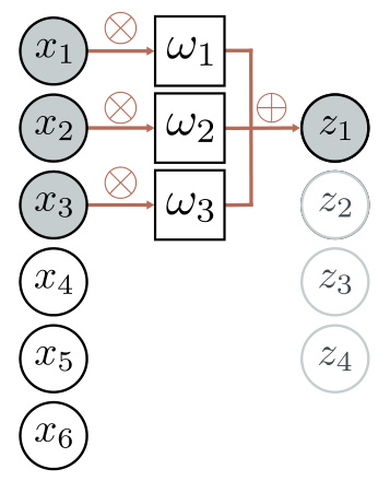
The formula computes each output from the previous, current, and subsequent input, which leaves the first output with no previous input and the final output with no subsequent one. There are two common approaches. Zero-padding assumes the input is zero outside its valid range; other possibilities are treating the input as circular or reflecting it at the boundaries. Valid convolution instead discards the output positions where the kernel exceeds the range of input positions. Valid convolution introduces no extra information at the edges of the input, at the cost of a representation that decreases in size.
Stride, kernel size, and dilation
Members of the larger family of convolution operations are distinguished by their stride, kernel size, and dilation rate.
Evaluating the output at every position is a stride of one; a stride of two shifts the kernel two positions between evaluations and creates roughly half the number of outputs.
Stride is therefore a downsampling mechanism as well as a hyperparameter of the kernel.
Kernel size can be increased to integrate over a larger area, but typically remains an odd number so that the kernel can be centered over the current position. Increasing it requires more weights.
Dilated or atrous convolution intersperses zeros between the weights. A kernel of size five becomes a dilated kernel of size three by setting its second and fourth elements to zero: information is still integrated from a region of five inputs, but only three weights are required. The number of zeros interspersed between the weights is the dilation rate.
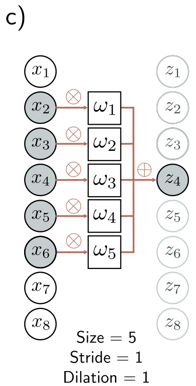
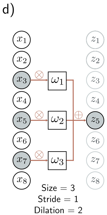
Work outward from the definition rather than memorizing a formula. With zero-padding and stride \(s\), the number of outputs is the number of input positions visited, roughly \(D/s\); with valid convolution and kernel size \(K\), the \(K-1\) positions where the kernel overhangs are discarded before that division. Dilation changes the span of the kernel and therefore the overhang, but never the number of weights.
Learning outcomes
- define-1d-convolution Define the 1D convolution operation with a shared kernel and compute its output.
- set-convolution-hyperparameters Choose kernel size, stride, padding, and dilation, and predict the resulting output size.
Concepts
- convolution-kernel the kernel \(\boldsymbol{\omega} = [\omega_1, \omega_2, \omega_3]^T\) holds the weights of the local weighted sum, and its size fixes how many inputs each output combines
- invariance-and-equivariance translating the input to a convolution translates its output identically, so the operation is equivariant to translation by construction
- padding zero-padding assumes out-of-range inputs are zero and preserves the output size, while valid convolution discards overhanging positions and shrinks it
- stride a stride of \(s\) evaluates the kernel every \(s\) positions and produces roughly \(1/s\) as many outputs
- dilated-convolution interspersing zeros between kernel weights integrates information over a larger region using the same number of weights
Layers, channels, and receptive fields
A convolutional layer computes its output by convolving the input, adding a bias \(\beta\), and passing each result through an activation function \(\mathrm{a}[\bullet]\). With kernel size three, stride one, and dilation rate one, the \(i^{th}\) hidden unit is
\[h_i = \mathrm{a}\Big[\beta + \sum_{j=1}^{3} \omega_j x_{i+j-2}\Big],\]
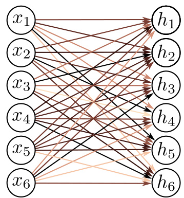
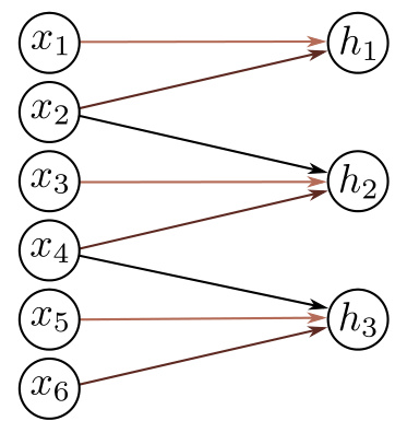
where the bias \(\beta\) and the kernel weights \(\omega_1, \omega_2, \omega_3\) are the trainable parameters, and with zero-padding the input \(x\) is treated as zero when out of range. This is a special case of a fully connected layer, which computes \(h_i = \mathrm{a}\big[\beta_i + \sum_{j=1}^{D} \omega_{ij} x_j\big]\). With \(D\) inputs and \(D\) hidden units, the fully connected layer has \(D^2\) weights and \(D\) biases; the convolutional layer uses three weights and one bias. A fully connected layer can reproduce the convolution exactly if most of its weights are set to zero and the others are constrained to be identical.
Channels
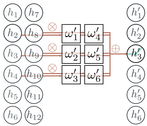
Applying a single convolution loses information: nearby inputs are averaged, and the ReLU clips results that are less than zero. Several convolutions are therefore computed in parallel, and each produces a new set of hidden variables termed a feature map or channel. With two kernels of size three and zero-padding, the first kernel produces \(h_1\) to \(h_6\) — the first channel — and the second, with different weights and a different bias, produces \(h_7\) to \(h_{12}\).
If the incoming layer has \(C_i\) channels and one kernel of size \(K\) is selected per channel, the hidden units in each output channel are a weighted sum over all \(C_i\) channels and \(K\) kernel entries, using a weight matrix \(\boldsymbol{\Omega} \in \mathbb{R}^{C_i \times K}\) and one bias. For \(C_o\) channels in the next layer, this requires \(\boldsymbol{\Omega} \in \mathbb{R}^{C_i \times C_o \times K}\) weights and \(\boldsymbol{\beta} \in \mathbb{R}^{C_o}\) biases. None of these counts depends on the spatial size of the input.
Receptive fields
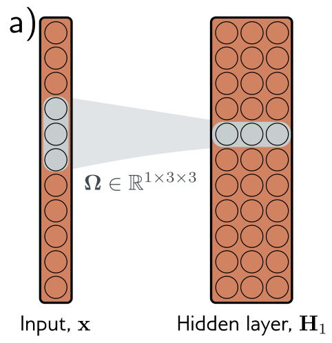
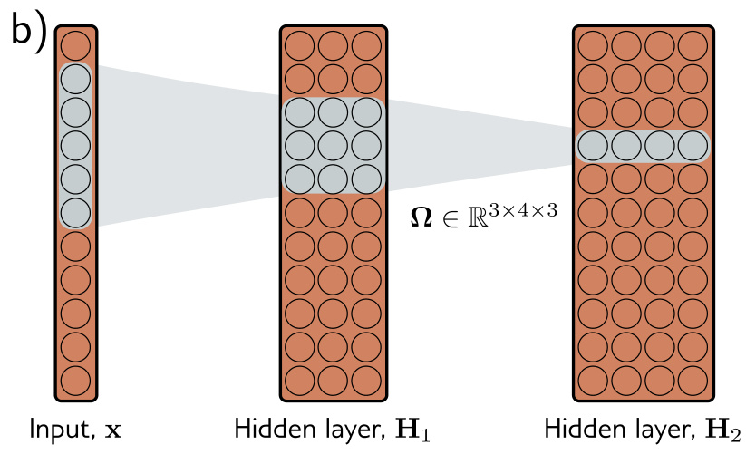
The receptive field of a hidden unit is the region of the original input that feeds into it. In a network where every convolutional layer has kernel size three and stride one, the units in the first layer take a weighted sum of the three closest inputs, so their receptive field has size three. The units in the second layer take a weighted sum of the three closest positions in the first layer, which are themselves weighted sums of three inputs, so their receptive field has size five. A third layer with kernel size three and stride two increases it to seven, and with an input of eleven dimensions, units at position three in a fourth layer have a receptive field covering the entire input.
Example: MNIST-1D
The MNIST-1D input \(\mathbf{x}\) is a 40D vector and the output \(\mathbf{f}\) is a 10D vector passed through a softmax layer. Three hidden layers are used. The fifteen channels of \(\mathbf{H}_1\) are each computed with kernel size three, stride two, and “valid” padding, giving nineteen spatial positions; \(\mathbf{H}_2\) and \(\mathbf{H}_3\) use the same settings, leaving four spatial positions and fifteen channels. Those sixty values are reshaped into a vector and mapped by a fully connected layer to the ten output activations.
The network was trained for 100,000 steps using SGD without momentum, a learning rate of 0.01, and a batch size of 100, on a dataset of 4,000 examples. The comparison is against a fully connected network with the same number of layers and hidden units — three hidden layers with 285, 135, and 60 hidden units. The convolutional network has 2,050 parameters and the fully connected network 59,065.
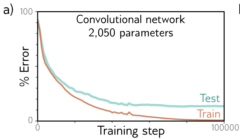
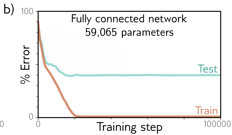
Both models fit the training data perfectly, so the gap is not one of capacity — and the fully connected model has enough flexibility to replicate the convolutional one exactly, but fails to do so. The discrepancy is probably not due to the difference in the number of parameters, since overparameterization usually improves performance. The likely explanation is the inductive bias: the architecture forces the network to process each position in the input in the same way, and the MNIST-1D data were created by starting with a template that is randomly translated. Equivalently, the convolutional structure can be considered a regularizer that applies an infinite penalty to most of the solutions a fully connected network can describe.
Learning outcomes
- build-conv-layers-and-channels Build a convolutional layer with multiple channels and count its parameters.
- reason-about-receptive-fields Trace the receptive field of a unit through a stack of convolutional layers.
- motivate-convolution Explain why fully connected layers fail on images, and state the invariance and equivariance a convolution buys.
Concepts
- convolutional-neural-network a convolutional layer is a fully connected layer whose weight matrix is banded and whose entries are tied, which is what reduces \(D^2 + D\) parameters to four
- channels-and-feature-maps several kernels applied in parallel produce several feature maps, so a layer mapping \(C_i\) to \(C_o\) channels holds \(C_i \times C_o \times K\) weights and \(C_o\) biases
- receptive-field the receptive field of a unit grows with depth — three, then five, then seven for kernel size three — which is how a local operator comes to integrate information from across the input
Two-dimensional convolutional networks
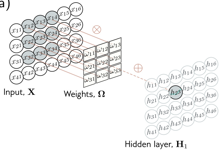
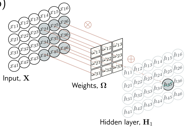
Convolutional networks for 1D data apply to financial time series, audio, and text, but they are more usually applied to 2D image data. The kernel is now a 2D object. A \(3 \times 3\) kernel \(\boldsymbol{\Omega} \in \mathbb{R}^{3 \times 3}\) applied to a 2D input of elements \(x_{ij}\) computes a single layer of hidden units \(h_{ij}\) as
\[h_{ij} = \mathrm{a}\Big[\beta + \sum_{m=1}^{3}\sum_{n=1}^{3} \omega_{mn}\, x_{i+m-2,\, j+n-2}\Big],\]
where \(\omega_{mn}\) are the entries of the convolutional kernel. This is a weighted sum over a square \(3 \times 3\) input region, and the kernel is translated both horizontally and vertically across the 2D input to create an output at each position.
Channels in two dimensions
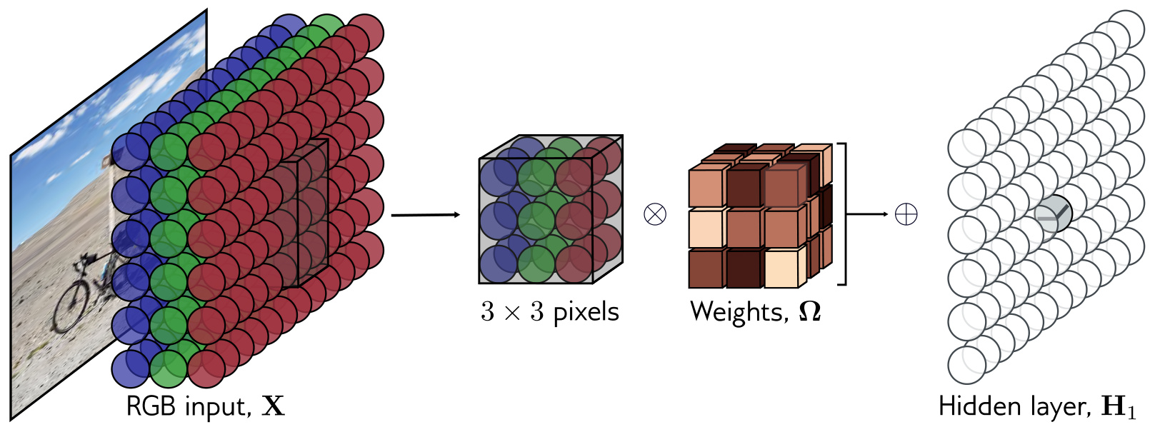
Often the input is an RGB image, treated as a 2D signal with three channels. A \(3 \times 3\) kernel then has \(3 \times 3 \times 3\) weights, applied to the three input channels at each of the \(3 \times 3\) positions, creating a 2D output the same height and width as the input under zero-padding. Multiple output channels are produced by repeating the process with different kernel weights and appending the results to form a 3D tensor. For kernel size \(K \times K\) and \(C_i\) input channels, each output channel is a weighted sum of \(C_i \times K \times K\) quantities plus one bias, so \(C_o\) output channels need \(C_i \times C_o \times K \times K\) weights and \(C_o\) biases.
Padding, stride, kernel size, and dilation carry over unchanged, applied one axis at a time. So does the parameter count’s independence from the input’s spatial size, which is what allows the same layer definition to be applied to images of different resolutions.
The architectural pattern
The MNIST-1D network of the previous section already shows the shape that 2D classification networks take: a sequence of convolutional layers that reduce the spatial extent of the representation while the channel count is held or increased, ending in a fully connected layer that integrates information from across the whole input and a softmax over classes. In that network the reduction came from stride-two convolutions with valid padding, taking forty positions to nineteen, then nine, then four.
Chapter 10 states the general form: typical convolutional networks consist of convolutional layers interspersed with layers that downsample by a factor of two, so that as a data example passes through the network the spatial dimensions usually decrease by factors of two and the channels increase by factors of two. Geometry is progressively exchanged for channel depth. At the end there are typically one or more fully connected layers that integrate information from across the entire input and create the desired output; if the output is itself an image, a mirrored decoder upsamples back to the original size.
Learning outcomes
- extend-to-2d Extend convolution to 2D images and read a standard image classification network.
- build-conv-layers-and-channels Build a convolutional layer with multiple channels and count its parameters.
Concepts
- convolution-kernel in 2D the kernel gains a second index, \(\omega_{mn}\), and spans all input channels, so a \(K \times K\) kernel over \(C_i\) channels holds \(C_i \times K \times K\) weights
- channels-and-feature-maps hidden units in a 2D network are stored as a tensor of height, width and channels, and each output channel is one kernel’s response across the whole spatial grid
Resampling and channel mixing
Three groups of operations change the shape of a representation. They are the plumbing from which the architectures in the rest of this unit are assembled.
Downsampling
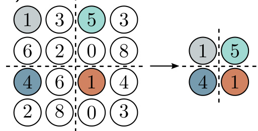
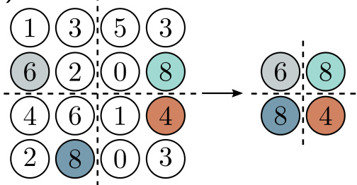
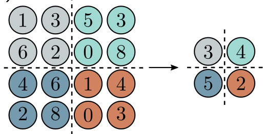
There are three main approaches to scaling down a 2D representation, taken here in the common case of scaling down both dimensions by a factor of two.
Sub-sampling retains every other position. Using a stride of two applies this simultaneously with the convolution operation, except that the discarded intermediate values are never computed.
Max pooling retains the maximum of the \(2 \times 2\) input values. This induces some invariance to translation: if the input is shifted by one pixel, many of these maximum values remain the same.
Mean pooling, or average pooling, averages the inputs.
For all approaches, downsampling is applied separately to each channel, so the output has half the width and height but the same number of channels.
Upsampling
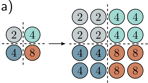
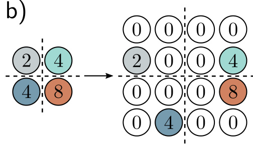
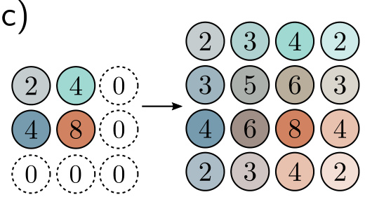
The simplest way to scale up a network layer to double the resolution is to duplicate all the channels at each spatial position four times. A second method is max unpooling, used where a max pooling operation was previously applied for downsampling: the values are distributed to the positions they originated from, which is where the maxima were. A third approach uses bilinear interpolation to fill in the missing values between the points where samples are available.
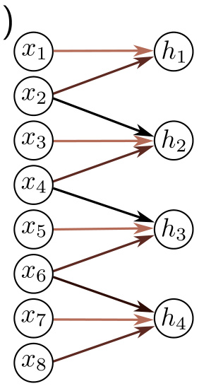
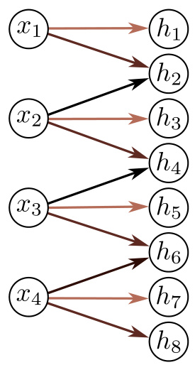
A fourth approach is roughly analogous to downsampling using a stride of two. In that method there were half as many outputs as inputs, and for kernel size three each output was a weighted sum of the three closest inputs. In transposed convolution this picture is reversed: there are twice as many outputs as inputs, and each input contributes to three of the outputs. Considering the associated weight matrix of this upsampling mechanism shows that it is the transpose of the matrix for the downsampling mechanism.
Changing the number of channels
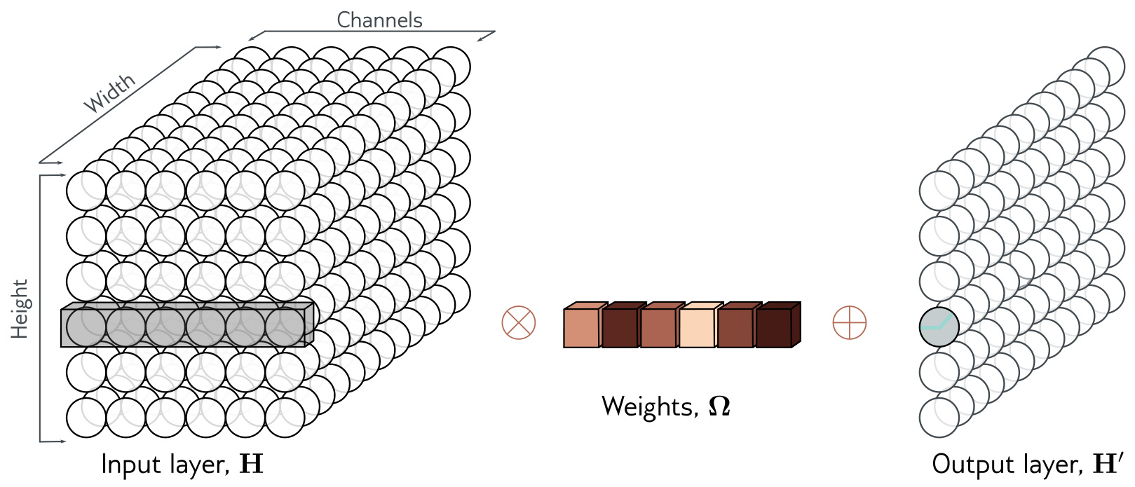
Sometimes the number of channels must change between one hidden layer and the next without further spatial pooling — usually so that the representation can be combined with another parallel computation, as in the residual architectures below. A convolution with kernel size one accomplishes this. Each element of the output layer is computed by taking a weighted sum of all the channels at the same position, and repeating this with different weights generates as many output channels as needed. The associated convolution weights have size \(1 \times 1 \times C_i \times C_o\), whence the name 1×1 convolution. Combined with a bias and activation function, it is equivalent to running the same fully connected network on the input channels at every position.
Learning outcomes
- change-resolution-and-channels Change spatial resolution and channel depth with pooling, upsampling, and 1x1 convolutions.
- reason-about-receptive-fields Trace the receptive field of a unit through a stack of convolutional layers.
Concepts
- downsampling-and-pooling sub-sampling, max pooling and mean pooling each halve width and height while leaving the channel count untouched, and are applied separately to every channel
- invariance-and-equivariance max pooling induces partial translation invariance, because a shift of one pixel leaves many of the per-block maxima unchanged
- upsampling-and-transposed-convolution duplication, max unpooling, bilinear interpolation and transposed convolution double the resolution, the last with a weight matrix that is the transpose of the strided downsampling matrix
- one-by-one-convolution a kernel of size one recombines the channels at each spatial position independently, which changes channel depth without touching the spatial dimensions
- channels-and-feature-maps channel count and spatial resolution are separately adjustable, which is what allows two branches of a network to be brought to a common shape
Vision tasks and their architectures
Three computer vision applications differ in what their output must be, and that difference drives the architecture.
Image classification
Much of the pioneering work on deep learning in computer vision used the ImageNet dataset, which contains 1,281,167 training images, 50,000 validation images, and 100,000 test images, every image labelled as belonging to one of 1000 possible categories. The input is a \(224 \times 224\) RGB image and the output a probability distribution over the 1000 classes. In 2011, before deep networks were applied, the state-of-the-art method classified the test images with about 25% errors for the correct class being in the top five suggestions.
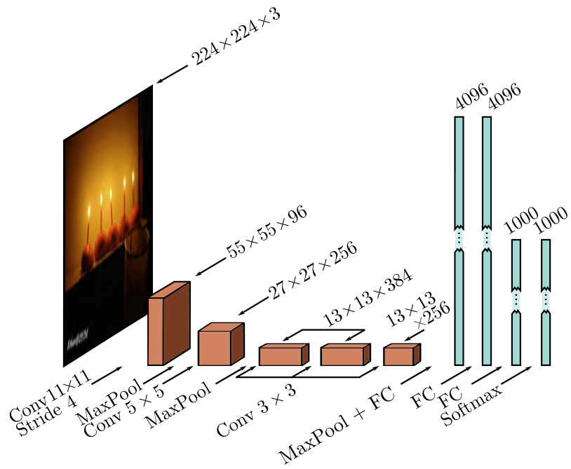
AlexNet, in 2012, was the first convolutional network to perform well on this task. It has eight hidden layers with ReLU activation functions, of which the first five are convolutional and the rest fully connected. It downsamples the input using an \(11 \times 11\) kernel with a stride of four to create 96 channels, downsamples again with a max pooling layer, applies a \(5 \times 5\) kernel to create 256 channels, then three more convolutional layers with kernel size \(3 \times 3\), eventually giving a \(13 \times 13\) representation with 256 channels. A final max-pooling layer yields a \(6 \times 6\) representation with 256 channels, resized into a vector of length 9,216 and passed through three fully connected layers containing 4096, 4096, and 1000 hidden units. The last layer is passed through the softmax function. The complete network contains about 60 million parameters, most of which are in the fully connected layers. Training used SGD with momentum coefficient 0.9 and batch size 128, dropout in the fully connected layers, an L2 (weight decay) regularizer, and a dataset augmented by a factor of 2048. It achieved a 16.4% top-5 error rate and a 38.1% top-1 error rate.
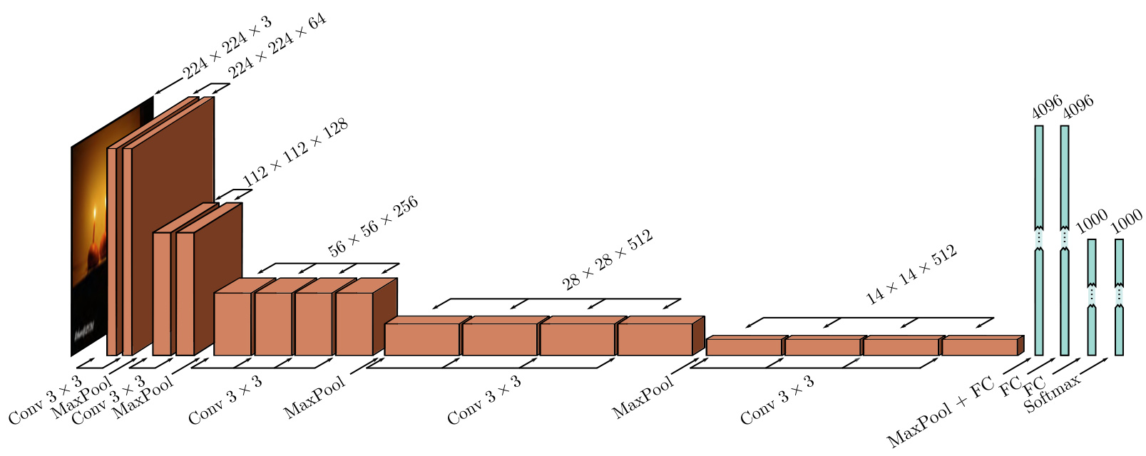
The VGG network achieved 6.8% top-5 and 23.7% top-1 error. It is similarly composed of interspersed convolutional and max pooling layers, where the spatial size of the representation gradually decreases but the number of channels increases, followed by three fully connected layers, and was also trained with data augmentation, weight decay, and dropout. Although there were minor differences in the training regime, the most important change between AlexNet and VGG was the depth of the network: VGG used 19 hidden layers and 144 million parameters.
Object detection
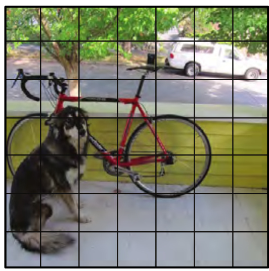
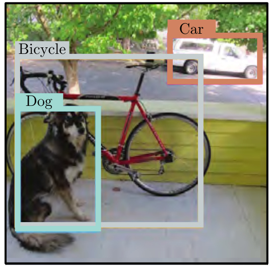
In object detection the goal is to identify and localize multiple objects within the image. An early method based on convolutional networks was You Only Look Once, or YOLO. Its input is a \(448 \times 448\) RGB image, passed through 24 convolutional layers that gradually decrease the representation size using max pooling operations while concurrently increasing the number of channels, similarly to the VGG network. The final convolutional layer is of size \(7 \times 7\) and has 1024 channels; this is reshaped to a vector, a fully connected layer maps it to 4096 values, and one further fully connected layer maps that representation to the output.
The output values encode which class is present at each of a \(7 \times 7\) grid of locations. For each location the output values also encode a fixed number of bounding boxes. Five parameters define each box: the x- and y-positions of the center, the height and width of the box, and the confidence of the prediction, which estimates the overlap between the predicted and ground truth bounding boxes. Training used momentum, weight decay, dropout, and data augmentation; transfer learning is employed, the network being initially trained on the ImageNet classification task and then fine-tuned for object detection. After the network is run, a heuristic process removes rectangles with low confidence and suppresses predicted boxes that correspond to the same object, so only the most confident one is retained.
Semantic segmentation
The goal of semantic segmentation is to assign a label to each pixel according to the object it belongs to, or no label if that pixel does not correspond to anything in the training database. In the network of Noh et al. (2015) the input is a \(224 \times 224\) RGB image and the output a \(224 \times 224 \times 21\) array containing the probability of each of 21 possible classes at each position.
The first part of the network is a smaller version of VGG containing thirteen rather than sixteen convolutional layers, downsizing the representation to size \(14 \times 14\). One more max pooling operation follows, then two fully connected layers mapping to two 1D representations of size 4096, which do not represent spatial position but combine information from across the whole image. Here the architecture diverges from VGG: another fully connected layer reconstitutes the representation into \(7 \times 7\) spatial positions and 512 channels, followed by a series of max unpooling layers and deconvolution layers, which are transposed convolutions in 2D and without the upsampling. Finally a \(1 \times 1\) convolution creates 21 channels representing the possible classes, and a softmax operation at each spatial position maps the activations to class probabilities. The downsampling side is referred to as an encoder and the upsampling side as a decoder, so networks of this type are called encoder-decoder networks or hourglass networks due to their shape.
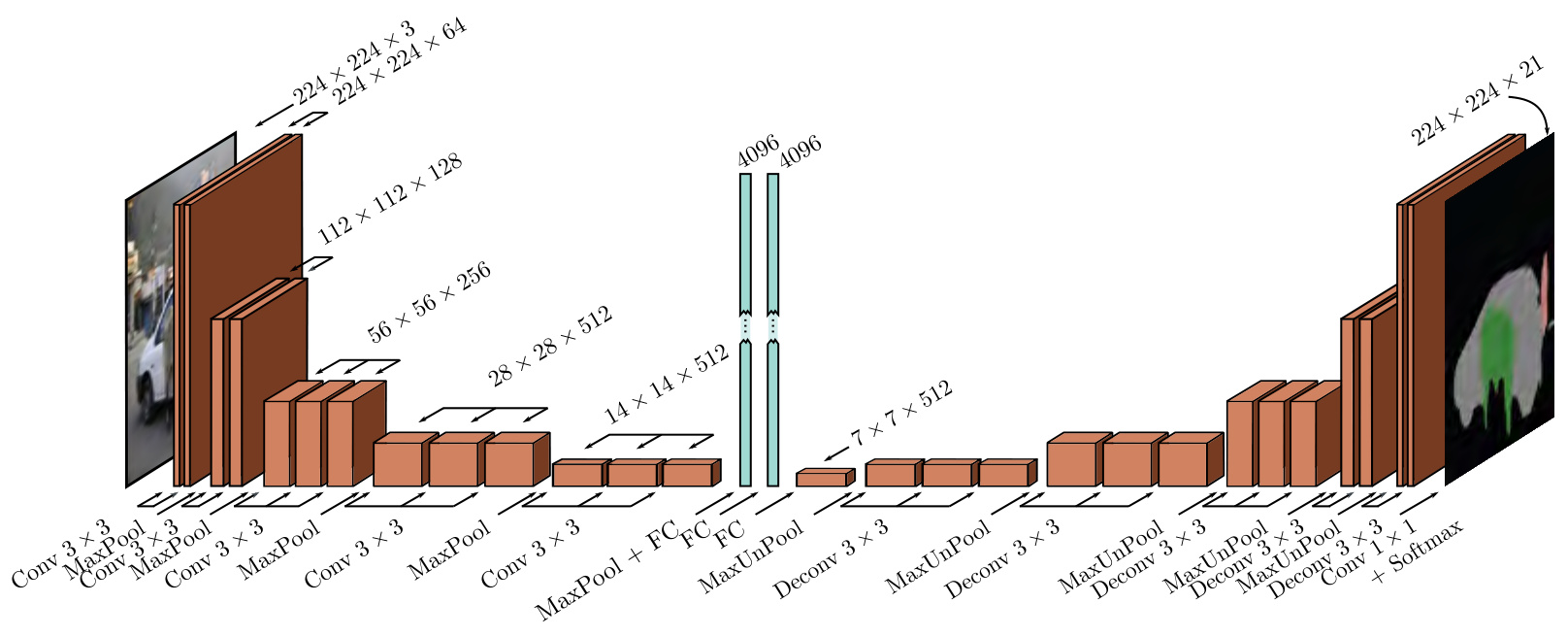
The low-resolution representation in the middle is what makes this architecture awkward: the receptive fields there are large and information is integrated from across the image, but the high-resolution detail needed for an accurate boundary must be carried through the bottleneck. Chapter 10 closes by noting that image classification performance was shown to improve as the network became deeper, but that increasing the network depth indefinitely does not continue to help: after a certain depth, the system becomes difficult to train.
Learning outcomes
- map-vision-tasks-to-architectures Match classification, object detection, and semantic segmentation to the architecture each needs.
- extend-to-2d Extend convolution to 2D images and read a standard image classification network.
- change-resolution-and-channels Change spatial resolution and channel depth with pooling, upsampling, and 1x1 convolutions.
Concepts
- alexnet eight hidden layers, five of them convolutional, about 60 million parameters, and a 16.4% top-5 ImageNet error rate
- vgg-network nineteen hidden layers of small \(3 \times 3\) kernels and max pooling, 144 million parameters, and a 6.8% top-5 error rate
- convolutional-neural-network the same convolutional backbone serves all three tasks, and what changes is the head and the resolution the architecture must preserve
- yolo-object-detection 24 convolutional layers reduce a \(448 \times 448\) image to a \(7 \times 7\) grid, at each cell of which a class, box coordinates and a confidence are predicted in a single pass
- encoder-decoder-network an encoder downsamples until information is integrated from across the image and a mirrored decoder upsamples back to per-pixel resolution
- upsampling-and-transposed-convolution max unpooling and deconvolution layers are what restore the decoder’s resolution, and a final \(1 \times 1\) convolution sets the channel count to the number of classes
The limits of sequential depth
Every network so far processes the data sequentially: each layer receives the previous layer’s output and passes the result to the next. A three-layer network is defined by
\[\mathbf{h}_1 = \mathbf{f}_1[\mathbf{x}, \boldsymbol{\phi}_1], \quad \mathbf{h}_2 = \mathbf{f}_2[\mathbf{h}_1, \boldsymbol{\phi}_2], \quad \mathbf{h}_3 = \mathbf{f}_3[\mathbf{h}_2, \boldsymbol{\phi}_3], \quad \mathbf{y} = \mathbf{f}_4[\mathbf{h}_3, \boldsymbol{\phi}_4],\]
which can equivalently be written as a series of nested functions, \(\mathbf{y} = \mathbf{f}_4\big[\mathbf{f}_3\big[\mathbf{f}_2[\mathbf{f}_1[\mathbf{x}, \boldsymbol{\phi}_1], \boldsymbol{\phi}_2], \boldsymbol{\phi}_3\big], \boldsymbol{\phi}_4\big]\).
In principle, layers can be added as freely as wanted, and the previous section saw that adding layers does improve performance: the nineteen-layer VGG network outperforms the eight-layer AlexNet. However, image classification performance decreases again as further layers are added. This is surprising since models generally perform better as more capacity is added. The decrease is present for both the training set and the test set, which implies that the problem is training deeper networks rather than the inability of deeper networks to generalize.
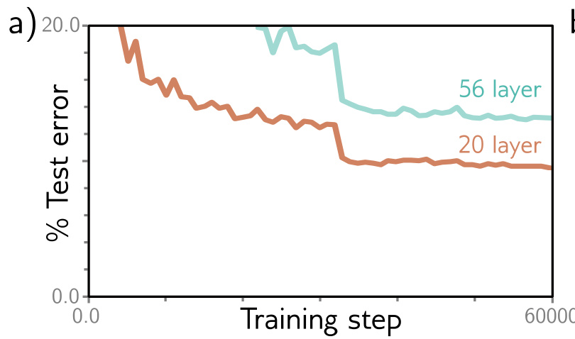
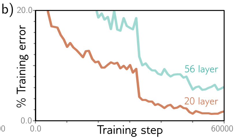
The phenomenon is not completely understood. One conjecture is that right after initialization the loss gradients change unpredictably when parameters in early network layers are modified. With appropriate initialization of the weights, the gradient of the loss with respect to those parameters will be reasonable — there are no exploding or vanishing gradients. However, the derivative assumes an infinitesimal change in the parameter, whereas optimization algorithms use a finite step size. Any reasonable choice of step size may move to a place with a completely different and unrelated gradient; the loss surface looks like an enormous range of tiny mountains rather than a single smooth structure that is easy to descend. Consequently, the algorithm does not make progress in the way that it does when the loss function gradient changes more slowly.
The conjecture is supported by empirical observations of gradients in networks with a single input and output. For a shallow network with 200 hidden units, the gradient \(\partial y / \partial x\) of the scalar output with respect to the scalar input changes relatively slowly as the input changes. For a deep network with 24 layers and 200 hidden units per layer, a tiny change in the input results in a completely different gradient. This is captured by the autocorrelation function of the gradient: nearby gradients are correlated for shallow networks, but this correlation quickly drops to zero for deep networks. This is termed the shattered gradients phenomenon.
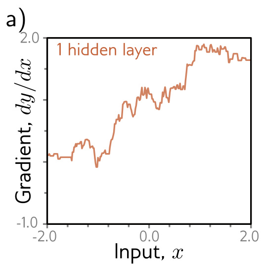
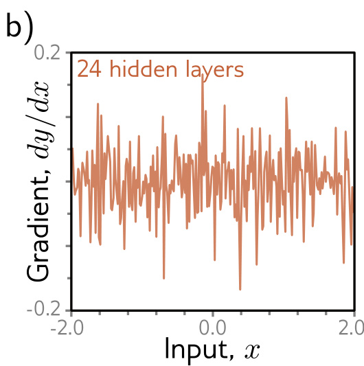
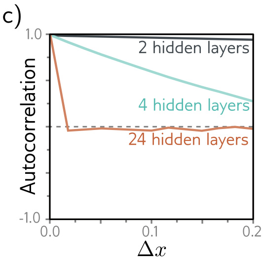
Shattered gradients presumably arise because changes in early network layers modify the output in an increasingly complex way as the network becomes deeper. The derivative of the output with respect to the first layer is
\[\frac{\partial \mathbf{y}}{\partial \mathbf{f}_1} = \frac{\partial \mathbf{f}_2}{\partial \mathbf{f}_1}\frac{\partial \mathbf{f}_3}{\partial \mathbf{f}_2}\frac{\partial \mathbf{f}_4}{\partial \mathbf{f}_3}.\]
When the parameters that determine \(\mathbf{f}_1\) are changed, all of the derivatives in this sequence are evaluated at slightly different locations, since layers \(\mathbf{f}_2, \mathbf{f}_3\), and \(\mathbf{f}_4\) are themselves computed from \(\mathbf{f}_1\). The updated gradient at each training example may therefore be completely different, and the loss function becomes badly behaved.
Learning outcomes
- diagnose-deep-network-training Explain why stacking more layers eventually makes training worse, not better.
Concepts
- sequential-processing in a sequential network every layer’s only input is the previous layer’s output, so the whole computation is one chain of nested functions and every early-layer derivative is a product along that chain
- shattered-gradients the autocorrelation of the gradient falls to zero as depth grows, so a finite gradient descent step lands at an unrelated gradient and optimization stops making progress
Residual connections
Residual or skip connections are branches in the computational path, whereby the input to each network layer \(\mathbf{f}[\bullet]\) is added back to the output. The residual network corresponding to the sequential network above is
\[\mathbf{h}_1 = \mathbf{x} + \mathbf{f}_1[\mathbf{x}, \boldsymbol{\phi}_1], \quad \mathbf{h}_2 = \mathbf{h}_1 + \mathbf{f}_2[\mathbf{h}_1, \boldsymbol{\phi}_2], \quad \mathbf{h}_3 = \mathbf{h}_2 + \mathbf{f}_3[\mathbf{h}_2, \boldsymbol{\phi}_3], \quad \mathbf{y} = \mathbf{h}_3 + \mathbf{f}_4[\mathbf{h}_3, \boldsymbol{\phi}_4],\]
where the first term on the right-hand side of each line is the residual connection. Each function \(\mathbf{f}_k\) learns an additive change to the current representation, from which it follows that their outputs must be the same size as their inputs. Each additive combination of the input and the processed output is known as a residual block or residual layer.
Unraveling
Substituting the expressions for the intermediate quantities gives a single function,
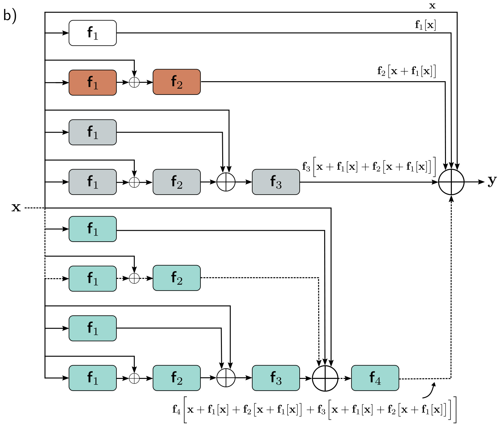
\[\mathbf{y} = \mathbf{x} + \mathbf{f}_1[\mathbf{x}] + \mathbf{f}_2\big[\mathbf{x} + \mathbf{f}_1[\mathbf{x}]\big] + \mathbf{f}_3\big[\mathbf{x} + \mathbf{f}_1[\mathbf{x}] + \mathbf{f}_2[\mathbf{x} + \mathbf{f}_1[\mathbf{x}]]\big] + \mathbf{f}_4\big[\cdots\big],\]
with the parameters omitted for clarity. The final network output is a sum of the input and four smaller networks, one corresponding to each line of the equation; one interpretation is that residual connections turn the original network into an ensemble of these smaller networks whose outputs are summed to compute the result. A complementary way of thinking about the same equation is that it creates sixteen paths of differing numbers of transformations between input and output.
The derivative
The first function \(\mathbf{f}_1[\mathbf{x}]\) occurs in eight of the sixteen paths, including as a direct additive term — a path length of one. The analogous derivative to the sequential case is
\[\frac{\partial \mathbf{y}}{\partial \mathbf{f}_1} = \mathbf{I} + \frac{\partial \mathbf{f}_2}{\partial \mathbf{f}_1} + \Big(\frac{\partial \mathbf{f}_3}{\partial \mathbf{f}_1} + \frac{\partial \mathbf{f}_2}{\partial \mathbf{f}_1}\frac{\partial \mathbf{f}_3}{\partial \mathbf{f}_2}\Big) + \Big(\frac{\partial \mathbf{f}_4}{\partial \mathbf{f}_1} + \frac{\partial \mathbf{f}_2}{\partial \mathbf{f}_1}\frac{\partial \mathbf{f}_4}{\partial \mathbf{f}_2} + \frac{\partial \mathbf{f}_3}{\partial \mathbf{f}_1}\frac{\partial \mathbf{f}_4}{\partial \mathbf{f}_3} + \frac{\partial \mathbf{f}_2}{\partial \mathbf{f}_1}\frac{\partial \mathbf{f}_3}{\partial \mathbf{f}_2}\frac{\partial \mathbf{f}_4}{\partial \mathbf{f}_3}\Big),\]
with one term for each of the eight paths. The identity term \(\mathbf{I}\) shows that changes in the parameters \(\boldsymbol{\phi}_1\) of the first layer contribute directly to changes in the network output, as well as indirectly through the other chains of derivatives of varying lengths. Gradients through shorter paths will in general be better behaved. Since both the identity term and various short chains of derivatives contribute to the derivative for each layer, networks with residual links suffer less from shattered gradients.
Order of operations
The additive functions must contain a nonlinear activation function, or the entire network will be linear. In a typical network layer the ReLU is at the end, so the output is non-negative; adopting that convention means each residual block can only increase the input values. It is therefore typical to change the order of operations so that the activation function is applied first, followed by the linear transformation. Sometimes there are several layers of processing within the residual block, but these usually terminate with a linear transformation. Blocks that start with a ReLU do nothing if the initial network input is negative, since the ReLU will clip the entire signal to zero; hence it is typical to start the network with a linear transformation rather than a residual block.
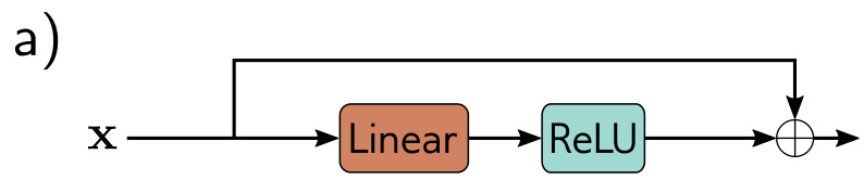

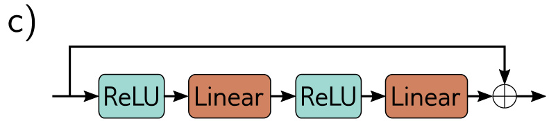
Adding residual connections roughly doubles the depth of a network that can be practically trained before performance degrades. Increasing the depth further requires attention to how the variance of the activations changes during the forward pass and how the gradient magnitudes change during the backward pass.
Learning outcomes
- build-residual-blocks Build a residual block and explain how skip connections restore gradient flow.
- diagnose-deep-network-training Explain why stacking more layers eventually makes training worse, not better.
Concepts
- residual-connections writing \(\mathbf{h}_k = \mathbf{h}_{k-1} + \mathbf{f}_k[\mathbf{h}_{k-1}]\) makes each branch learn an additive correction to the identity, and unraveling the stack exposes an ensemble of paths of differing length
- shattered-gradients the identity term in the residual derivative gives every layer a direct route to the output, so gradients need not propagate through long chains and are better behaved
- pre-activation-residual-block ordering the block activation-then-linear lets it add negative as well as positive quantities, which a block ending in a ReLU cannot do
Batch normalization
Careful initialization matters because without it the magnitudes of the intermediate values in the forward pass, and the gradients in the backward pass, increase or decrease exponentially. He initialization achieves stability for ReLU activations by initializing the biases \(\boldsymbol{\beta}\) to zero and choosing normally distributed weights \(\boldsymbol{\Omega}\) with mean zero and variance \(2/D_h\), where \(D_h\) is the number of hidden units in the previous layer.
In a residual network, vanishing values and gradients are not a concern, since each layer contributes directly to the output. However, even with He initialization inside the residual block, the values in the forward pass increase exponentially with depth. The result of the processing in the residual block is added back to the input, and each branch has some uncorrelated variability, so the overall variance increases when they are recombined. With ReLU activations and He initialization, the expected variance is unchanged by the processing in each block; consequently, when it is recombined with the input, the variance doubles, growing exponentially with the number of residual blocks. This limits the possible network depth before floating point precision is exceeded in the forward pass, and a similar argument applies to the gradients in the backward pass.
One approach that would stabilize both passes is to use He initialization and then multiply the combined output of each residual block by \(1/\sqrt{2}\) to compensate for the doubling. It is more usual to use batch normalization.



The operation
Batch normalization, or BatchNorm, shifts and rescales each activation \(h\) so that its mean and variance across the batch \(\mathcal{B}\) become values that are learned during training. First the empirical mean \(m_h\) and standard deviation \(s_h\) are computed:
\[m_h = \frac{1}{|\mathcal{B}|}\sum_{i \in \mathcal{B}} h_i, \qquad s_h = \sqrt{\frac{1}{|\mathcal{B}|}\sum_{i \in \mathcal{B}} (h_i - m_h)^2},\]
where all quantities are scalars. These statistics standardize the batch activations to have mean zero and unit variance,
\[h_i \leftarrow \frac{h_i - m_h}{s_h + \epsilon} \qquad \forall i \in \mathcal{B},\]
where \(\epsilon\) is a small number that prevents division by zero if \(h_i\) is the same for every member of the batch and \(s_h = 0\). Finally the normalized variable is scaled by \(\gamma\) and shifted by \(\delta\):
\[h_i \leftarrow \gamma h_i + \delta \qquad \forall i \in \mathcal{B}.\]
After this operation the activations have mean \(\delta\) and standard deviation \(\gamma\) across all members of the batch, and both quantities are learned during training.
Batch normalization is applied independently to each hidden unit. In a standard neural network with \(K\) layers each containing \(D\) hidden units there would be \(KD\) learned offsets \(\delta\) and \(KD\) learned scales \(\gamma\). In a convolutional network the normalizing statistics are computed over both the batch and the spatial position, so with \(K\) layers each containing \(C\) channels there are \(KC\) offsets and \(KC\) scales.
At test time there is no batch from which to gather statistics. To resolve this, \(m_h\) and \(s_h\) are calculated across the whole training dataset rather than just a batch and frozen in the final network. A network evaluated with batch statistics and one evaluated with the frozen statistics are not the same function.
Costs and benefits
Batch normalization makes the network invariant to rescaling the weights and biases that contribute to each activation: if these are doubled, the activations also double, the estimated standard deviation \(s_h\) doubles, and the standardization compensates for these changes. Consequently there is a large family of weights and biases that all produce the same effect. It also adds two parameters, \(\gamma\) and \(\delta\), at every hidden unit. It therefore both creates redundancy in the weights and biases and adds extra parameters to compensate for that redundancy. Against that:
Stable forward propagation. With the offsets \(\delta\) initialized to zero and the scales \(\gamma\) to one, each output activation has unit variance. In a residual network the variance must still increase as a new source of variation is added at each layer, but it increases linearly: the \(k^{th}\) layer adds one unit of variance to the existing variance of \(k\).
A side effect at initialization is that later layers make a smaller change to the overall variation than earlier ones, so the network is effectively less deep at the start of training. As training proceeds it can increase the scales \(\gamma\) in later layers and control its own effective depth.
Higher learning rates. Empirical studies and theory both show that batch normalization makes the loss surface and its gradient change more smoothly — that is, it reduces shattered gradients — so higher learning rates can be used because the surface is more predictable.
Regularization. BatchNorm injects noise, because the normalization depends on the batch statistics. The activations for a given training example are normalized by an amount that depends on the other members of the batch and is different at each training iteration.
Learning outcomes
- apply-batch-normalization Apply batch normalization and state what it fixes and what it costs.
- build-residual-blocks Build a residual block and explain how skip connections restore gradient flow.
Concepts
- residual-connections because a block’s output is added back to an uncorrelated input of equal variance, each residual addition doubles the variance and the growth is exponential in the number of blocks
- batch-normalization standardizing each activation by its batch mean and standard deviation and then applying a learned scale and offset turns that exponential variance growth into linear growth
- shattered-gradients normalization makes the loss surface and its gradient change more smoothly, which is what permits the larger learning rates
Common residual architectures
Residual connections are now a standard part of deep learning pipelines. Three architectures put the same principle to different uses.
ResNet
Residual blocks were first used in convolutional networks for image classification; the resulting networks are known as residual networks, or ResNets. In a ResNet, each residual block contains a batch normalization operation, a ReLU activation function, and a convolutional layer, followed by the same sequence again before being added back to the input. Trial and error have shown that this order of operations works well for image classification.
For very deep networks the number of parameters may become undesirably large. Bottleneck residual blocks make more efficient use of parameters using three convolutions: the first has a \(1 \times 1\) kernel and reduces the number of channels, the second is a regular \(3 \times 3\) kernel, and the third is another \(1 \times 1\) kernel to increase the number of channels back to the original amount. Information is still integrated over a \(3 \times 3\) pixel area, using fewer parameters.
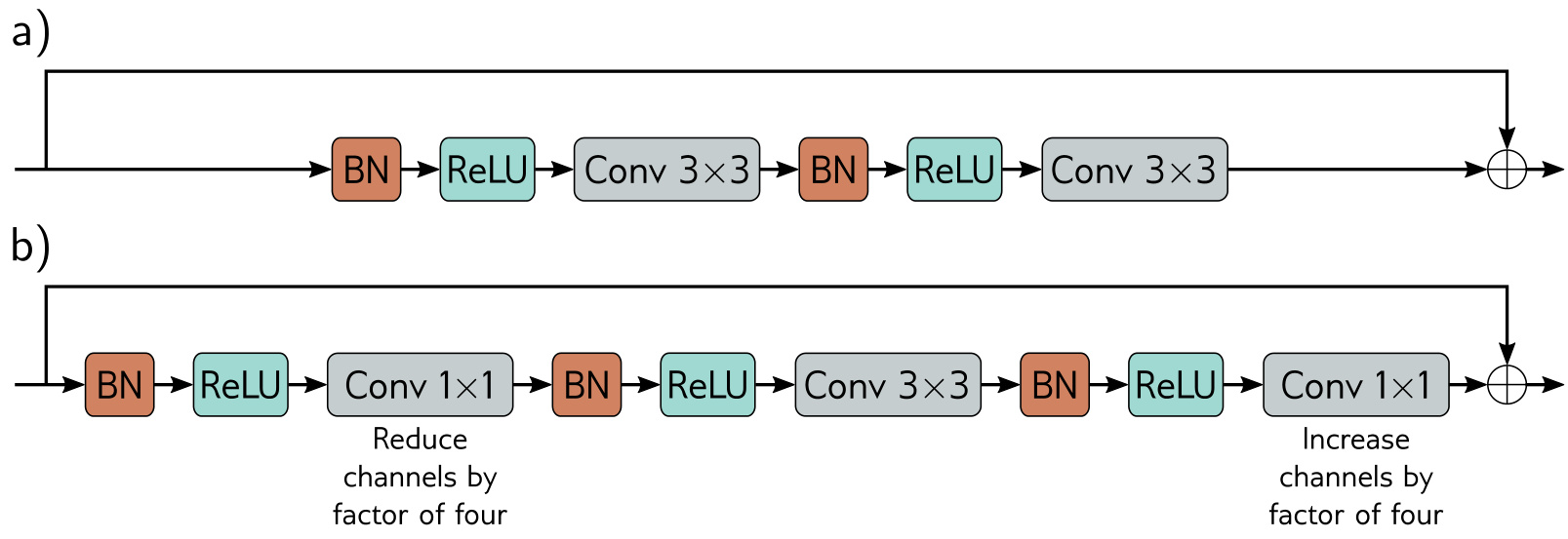
The ResNet-200 model contains 200 layers and was used for image classification on ImageNet. The architecture resembles AlexNet and VGG but uses bottleneck residual blocks instead of vanilla convolutional layers. As with those networks, decreases in spatial resolution are periodically interspersed with simultaneous increases in the number of channels; the resolution is decreased between adjacent ResNet blocks using convolutions with stride two, and channels are added either by appending zeros to the representation or by applying an extra \(1 \times 1\) convolution. At the start of the network is a \(7 \times 7\) convolutional layer followed by a downsampling operation. At the end, a fully connected layer maps the block to a vector of length 1000, passed through a softmax layer. ResNet-200 achieved a 4.8% error rate for the correct class being in the top five and 20.1% for identifying the correct class correctly. This compared favourably with AlexNet (16.4%, 38.1%) and VGG (6.8%, 23.7%) and was one of the first networks to exceed human performance, estimated at 5.1% for being in the top five guesses.
DenseNet
Residual blocks receive the output from the previous layer, modify it, and add it back to the original input. An alternative is to concatenate the modified and original signals. This increases the representation size in terms of channels, but an optional subsequent linear transformation can map back to the original size — a \(1 \times 1\) convolution for a convolutional network — which allows the model to add the representations together, take a weighted sum, or combine them in a more complex way.
The DenseNet architecture uses concatenation so that the input to a layer comprises the concatenated outputs from all previous layers. These are processed to create a new representation that is itself concatenated with the previous representation and passed to the next layer. The concatenation means there is a direct contribution from earlier layers to the output, so the loss surface behaves reasonably.
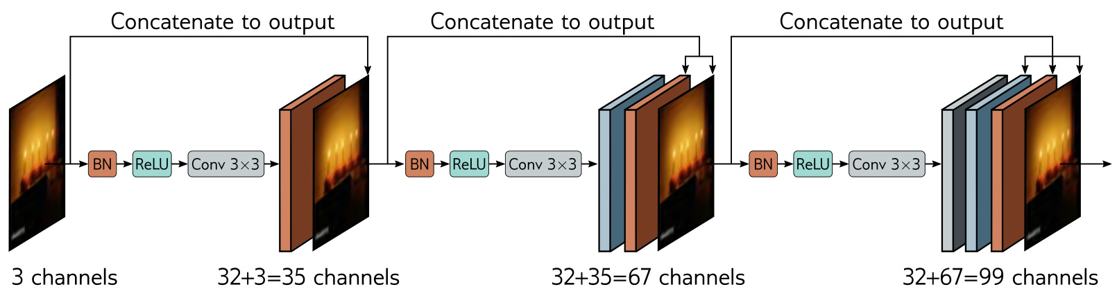
In practice this can only be sustained for a few layers, because the number of channels — and hence the number of parameters required to process them — becomes increasingly large. Applying a \(1 \times 1\) convolution to reduce the number of channels before the next \(3 \times 3\) convolution alleviates the problem. In a convolutional network the input is periodically downsampled; concatenation across the downsampling makes no sense since the representations have different spatial sizes, so the chain of concatenation is broken at this point and a smaller representation starts a new chain. DenseNet performs competitively with ResNet models on image classification, and can perform better for a comparable parameter count, presumably because it can reuse processing from earlier layers more flexibly.
U-Nets and hourglass networks
The encoder–decoder segmentation network of the previous section has one drawback: the low-resolution representation in the middle of the network must “remember” the high-resolution details to make the final result accurate. This is unnecessary if residual connections transfer the representations from the encoder to their partner in the decoder.
The U-Net is an encoder-decoder architecture where the earlier representations are concatenated to the later ones. The original implementation used “valid” convolutions, so the spatial size decreases by two pixels each time a \(3 \times 3\) convolutional layer is applied; the upsampled version is therefore smaller than its counterpart in the encoder, which must be cropped before concatenation. Subsequent implementations have used zero-padding, where this cropping is unnecessary. The U-Net is completely convolutional, so after training it can be run on an image of any size.
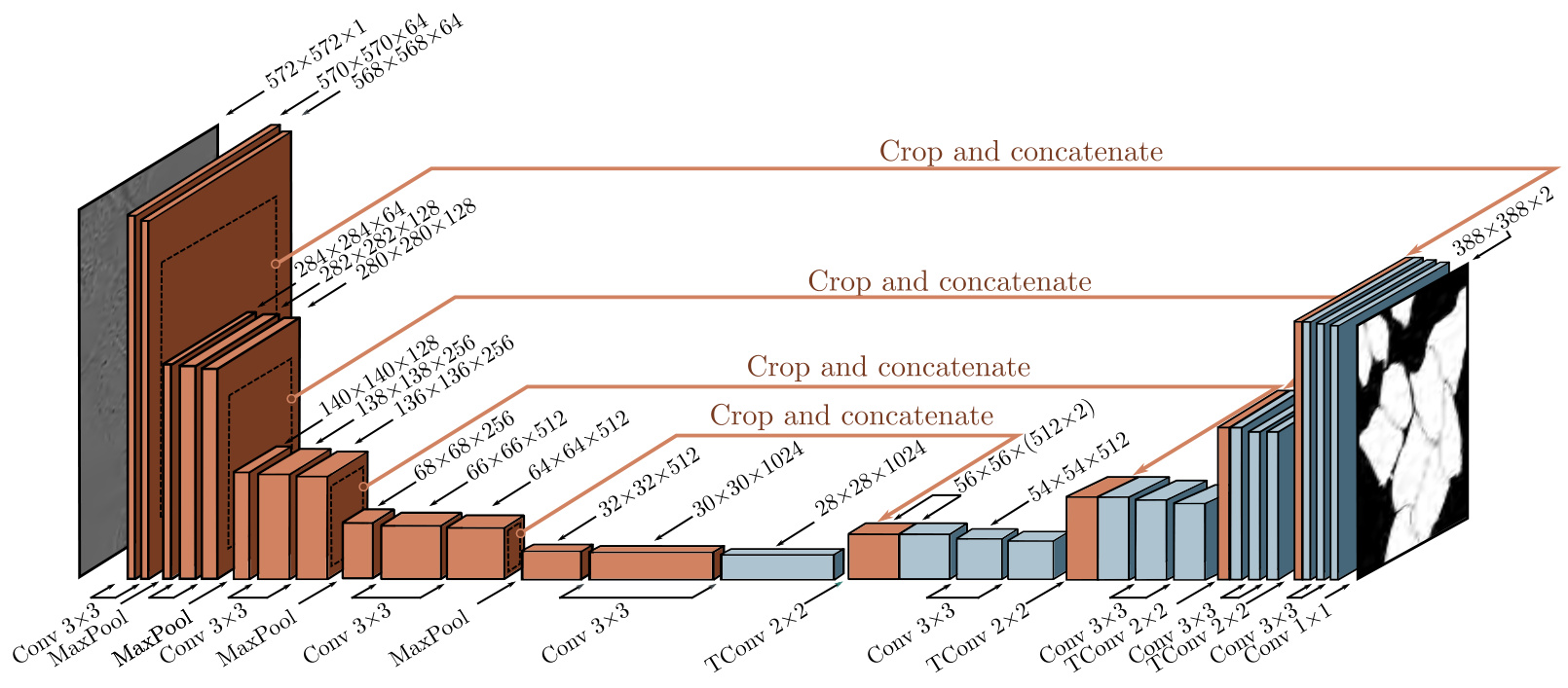
The U-Net was intended for segmenting medical images but has found many other uses in computer graphics and vision. Hourglass networks are similar but apply further convolutional layers in the skip connections and add the result back to the decoder rather than concatenating it. A series of these models form a stacked hourglass network that alternates between considering the image at local and global levels. Such networks are used for pose estimation: the system is trained to predict one “heatmap” for each joint, and the estimated position is the maximum of each heatmap.
Learning outcomes
- compare-residual-architectures Compare ResNet, DenseNet, and U-Net as different uses of the same skip principle.
- map-vision-tasks-to-architectures Match classification, object detection, and semantic segmentation to the architecture each needs.
- change-resolution-and-channels Change spatial resolution and channel depth with pooling, upsampling, and 1x1 convolutions.
Concepts
- residual-connections the same additive shortcut appears at the scale of a two-convolution block in ResNet and at the scale of a whole encoder stage in an hourglass network
- bottleneck-residual-block a \(1 \times 1\) convolution reduces the channels, a \(3 \times 3\) does the spatial work, and a second \(1 \times 1\) restores the channel count so the result can be added back
- densenet concatenating rather than adding gives every layer the outputs of all preceding layers, and the resulting channel growth is controlled by \(1 \times 1\) convolutions and broken at each downsampling
- u-net long skips carry each encoder scale’s high-resolution representation to the matching decoder scale, which removes the need for the bottleneck to retain spatial detail
- stacked-hourglass-network chaining encoder-decoder blocks, with convolutions in the skip paths whose output is added rather than concatenated, alternates local and global processing to regress one heatmap per joint
Why residual networks perform well
Residual networks allow much deeper networks to be trained; it is possible to extend the ResNet architecture to 1000 layers and still train effectively. The improvement in image classification performance was initially attributed to the additional network depth, but two pieces of evidence contradict this viewpoint.
Shallower, wider residual networks sometimes outperform deeper, narrower ones with a comparable parameter count.
Better performance can sometimes be achieved with a network with fewer layers but more channels per layer, which depth alone does not explain.
There is evidence that the gradients during training do not propagate effectively through very long paths in the unraveled network.
In effect, a very deep network may act more like a combination of shallower networks.
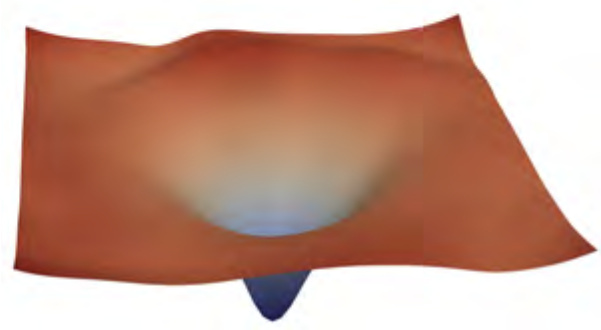
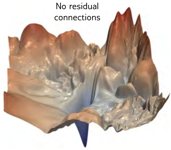
The current view is that residual connections add some value of their own, as well as allowing deeper networks to be trained. This perspective is supported by the fact that the loss surfaces of residual networks around a minimum tend to be smoother and more predictable than those for the same network when the skip connections are removed. This may make it easier to learn a good solution that generalizes well.
The two accounts cover different observations, and it is worth being precise about which.
The loss surface account explains why the same architecture trains at all: the surface around a minimum is smooth and predictable rather than chaotic, so a finite-step optimizer makes progress, and a minimum in a smooth basin is robust to minor errors in the parameters.
The ensemble account explains the two observations above: that width can substitute for depth, and that the gradients do not traverse the longest paths. If most of the effective computation happens along relatively short paths, a 200-layer residual network is not doing 200 layers’ worth of sequential processing.
Neither account is a claim that raw depth is responsible. Plain sequential networks of the same depth train worse, as the CIFAR-10 comparison in an earlier section showed.
Learning outcomes
- explain-residual-success Explain why residual networks work, beyond the claim that they are deeper.
- build-residual-blocks Build a residual block and explain how skip connections restore gradient flow.
- apply-batch-normalization Apply batch normalization and state what it fixes and what it costs.
Concepts
- residual-connections adding the processed representation back to its own input makes each layer contribute to the output directly as well as indirectly, so propagating gradients through many layers is not mandatory
- shattered-gradients both residual links and batch normalization make the loss surface smoother, which is the mechanism by which they remove the shattered-gradients failure
Key ideas from this unit
Key ideas
A convolutional layer is a fully connected layer with most weights set to zero and the rest tied, and its parameter count does not depend on the input’s spatial size.
That constraint is the inductive bias: on MNIST-1D it reaches 17% test error with 2,050 parameters where an unconstrained network with 59,065 parameters reaches 40%.
Convolution is equivariant to translation by construction, and pooling on top of it produces partial invariance.
The symmetry is a property of the architecture, so it does not have to be estimated from data.
Kernel size, stride, padding, and dilation determine the output geometry, and depth determines the receptive field.
A local operator becomes a global one only through composition — three inputs, then five, then seven for kernel size three.
Pooling, transposed convolution, and the \(1 \times 1\) convolution are what let a network change resolution and channel depth independently.
Classification pools resolution away, segmentation must restore it, and bottleneck blocks trade channel depth for parameters.
Adding layers to a sequential network eventually increases the training error, not just the test error.
The failure is one of optimization: gradient autocorrelation falls to zero with depth, so a finite step lands at an unrelated gradient.
Writing \(\mathbf{h}_k = \mathbf{h}_{k-1} + \mathbf{f}_k[\mathbf{h}_{k-1}]\) puts an identity term in the derivative and roughly doubles the trainable depth.
Unraveling the same equation shows a sum over paths of differing length, which is why gradients need not survive the longest chain.
Each residual addition doubles the activation variance, and batch normalization reduces that growth from exponential to linear.
It costs a train/test discrepancy resolved by frozen dataset statistics, plus two parameters per hidden unit and a redundancy in the weights.
ResNet adds the shortcut, DenseNet concatenates it, and the U-Net carries it across the whole architecture.
The choice follows the task: additive bottleneck blocks for classification, concatenation for feature reuse, long skips for per-pixel output.
The evidence favours a smoother loss surface and ensemble-like behaviour over shallow paths, not depth as such.
Wider shallow residual networks can match deeper narrow ones, and plain networks of the same depth train worse.
This closes Basics to Machine Learning. Across its three units the recipe never changed: a parameterized model, a loss derived from a likelihood, gradient-based optimization, and a measurement discipline separating training error from generalization. What changed was the model family — a straight line, then a shallow network, then a deep one, then a convolutional residual network — and the machinery required to make each family trainable.
References
- Understanding Deep Learning, Simon Prince, 2026 — Link — Pages 175-199, 200-220