Convnets

Basics to Machine Learning · v1.1.27

2026-09-22 13:30:36

Vision as a learning problem

What carries over, and what changes

The previous unit assembled a complete supervised pipeline.

• a loss derived as a negative log-likelihood
• minibatch SGD with momentum or Adam, and backpropagation
• explicit and implicit regularizers

All of it applies here unchanged. What changes is the model family.

Nothing about optimization is revised in this unit. The single move is to replace the fully connected layer with one that respects the structure of an image.

Three tasks in vision

The task

1. Image classification — one label for the whole image
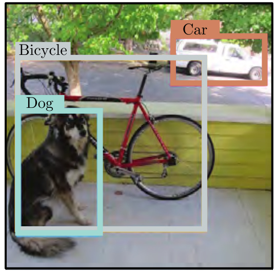
2. Object detection — a class and a box for each object
3. Semantic segmentation — a label at every pixel

The output

1. A distribution over classes
2. A list of boxes, each with a class and a confidence
3. An image-sized array of class probabilities

What the output must be decides the architecture.

Images are spatial

An image is not a bag of numbers. Three properties of the data are ignored by a fully connected layer:

• the input is two-dimensional, and position carries meaning
• nearby pixels are statistically related
• the interpretation is stable under geometric transformation

A tree is a tree wherever it appears in the frame.

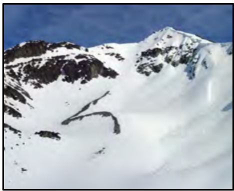
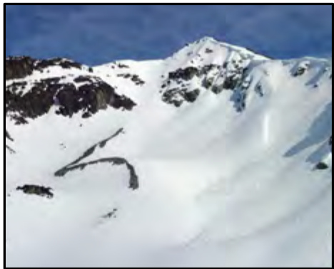
Invariance

A function \(\mathbf{f}\) is invariant to \(\mathbf{t}\) when \(\mathbf{f}\big[\mathbf{t}[\mathbf{x}]\big] = \mathbf{f}[\mathbf{x}]\)

A photograph of a mountain.

The same scene, horizontally shifted.

The output does not move when the input does.

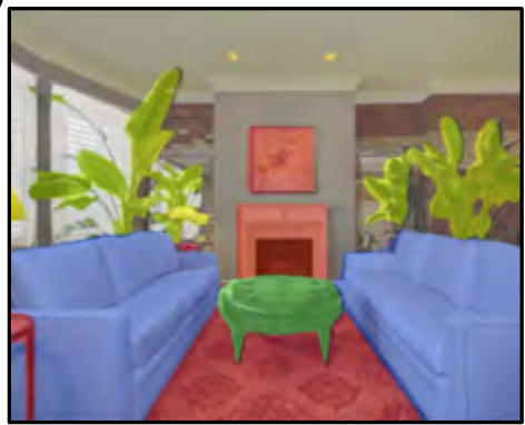
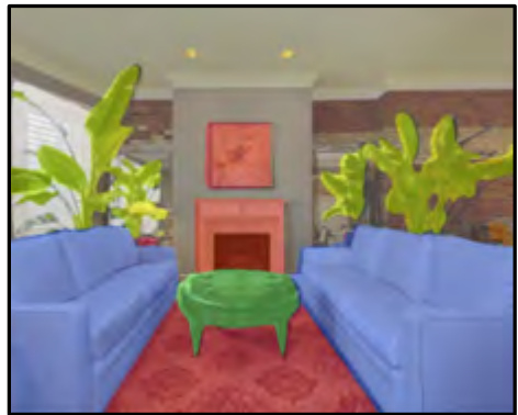
Equivariance

A function \(\mathbf{f}\) is equivariant to \(\mathbf{t}\) when \(\mathbf{f}\big[\mathbf{t}[\mathbf{x}]\big] = \mathbf{t}\big[\mathbf{f}[\mathbf{x}]\big]\)

One label per pixel.

The overlay for a translated input.

The output moves exactly as the input does.

Which task wants which

Classification wants invariance

• Both photographs are “mountain”
• A shift must not change the label
• \(\mathbf{f}[\mathbf{t}[\mathbf{x}]] = \mathbf{f}[\mathbf{x}]\)

Segmentation wants equivariance

• Shift the image, and the overlay shifts with it
• A label belongs to a position
• \(\mathbf{f}[\mathbf{t}[\mathbf{x}]] = \mathbf{t}[\mathbf{f}[\mathbf{x}]]\)

Neither implies the other: an equivariant output moves, an invariant one does not.

Convolutional layers are equivariant to translation by construction. Invariance for a classifier comes from the pooling placed on top, and only partially — a convolutional classifier is not exactly invariant to translation.

The cost of a fully connected layer

A \(224 \times 224\) RGB image is \(150{,}528\) input dimensions.

• Hidden layers are generally at least as wide as the input
• One such layer therefore needs \(150{,}528^2\) weights

\[\approx 2.2 \times 10^{10} \text{ parameters, in a single layer}\]

Prohibitive before training has even been considered.

Two objections beyond cost

Structure is discarded

• Every pair of inputs is treated alike
• Permuting all pixels identically would change nothing about training

Symmetry must be learned

• Shifting an image changes every input
• The pattern signifying a tree is learned separately at every position

Possible in principle, and wasteful in every respect.

A fully connected network could in principle represent a translation-equivariant function. It would have to discover, from data alone, that the weights at one position should equal the weights at every other. Convolution asserts that instead of estimating it.

Convolution in one dimension

The operation

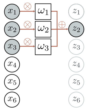
Each output is a weighted sum of nearby inputs, with the same weights at every position:

\[z_i = \omega_1 x_{i-1} + \omega_2 x_i + \omega_3 x_{i+1}\]

• \(\boldsymbol{\omega} = [\omega_1, \omega_2, \omega_3]^T\) is the kernel, or filter
• The number of weights is the kernel size
• The kernel is the layer’s only parameter set

Strictly this is a cross-correlation: a true convolution flips the weights relative to the input, switching \(x_{i-1}\) and \(x_{i+1}\). The incorrect definition is the usual convention in machine learning.

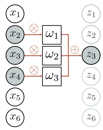
The same weights, one position on

\(z_2 = \omega_1 x_1 + \omega_2 x_2 + \omega_3 x_3\)

\(z_3 = \omega_1 x_2 + \omega_2 x_3 + \omega_3 x_4\)

Translating the input translates the output identically — equivariance, by construction.

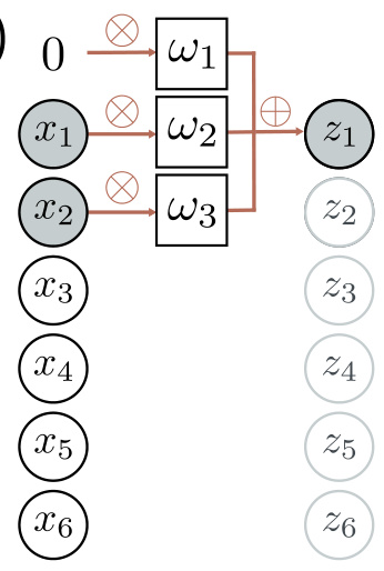
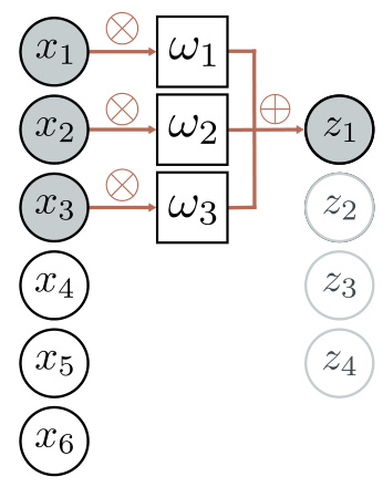
The boundary

Zero-padding — out-of-range inputs taken as zero, output size kept.

Valid — overhanging positions discarded, output shrinks.

The first output has no previous input, the last no subsequent one.

Stride and kernel size

Stride

• Stride one evaluates at every position
• Stride \(s\) advances \(s\) positions between evaluations
• Roughly \(1/s\) as many outputs — downsampling for free

Kernel size

• A larger kernel integrates over a larger region
• Usually odd, so the kernel centres on its position
• Every extra position costs a weight

Dilation

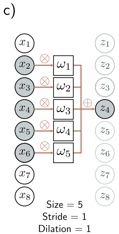
Size five, dilation one.

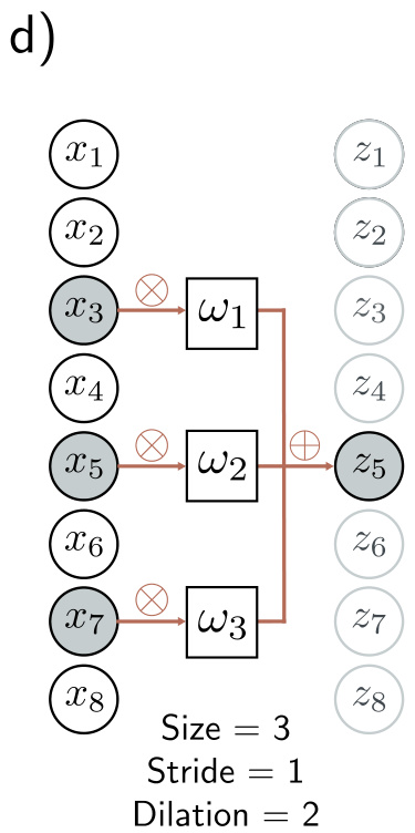
Size three, dilation two.

Two readings: sample every second input, or zero-pad the kernel.

Also termed atrous convolution. The dilation rate is the number of zeros between adjacent weights. Dilation changes the span of the kernel, and so the overhang at the boundary, but never the number of weights.

Output size and model size

A kernel of size \(K\) at dilation rate \(r\) spans \(K' = r(K-1)+1\) positions.

Output size

Input length \(D\), padding \(p\) each side, stride \(s\):

\[D_{out} = \left\lfloor \frac{D + 2p - K'}{s} \right\rfloor + 1\]

Valid convolution: \(p = 0\). Size-preserving: \(p = (K'-1)/2\).

Model size

One kernel and one bias:

\[K + 1\]

The \(K\) kernel weights and the bias, whatever \(D\), \(p\), \(s\) or \(r\) may be.

Model size is independent of \(D\), and of the dilation rate.

The convolutional layer

A convolution, a bias, and an activation function:

\[h_i = \mathrm{a}\Big[\beta + \sum_{j=1}^{3} \omega_j\, x_{i+j-2}\Big]\]

The fully connected layer, for comparison:

\[h_i = \mathrm{a}\Big[\beta_i + \sum_{j=1}^{D} \omega_{ij}\, x_j\Big]\]

Four trainable parameters against \(D^2 + D\).

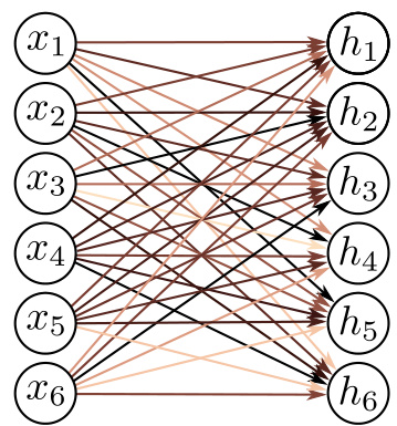
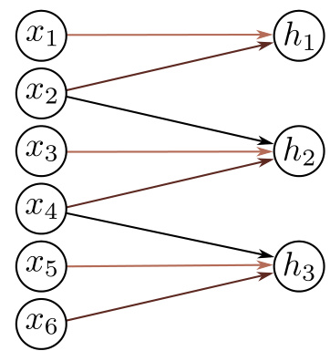
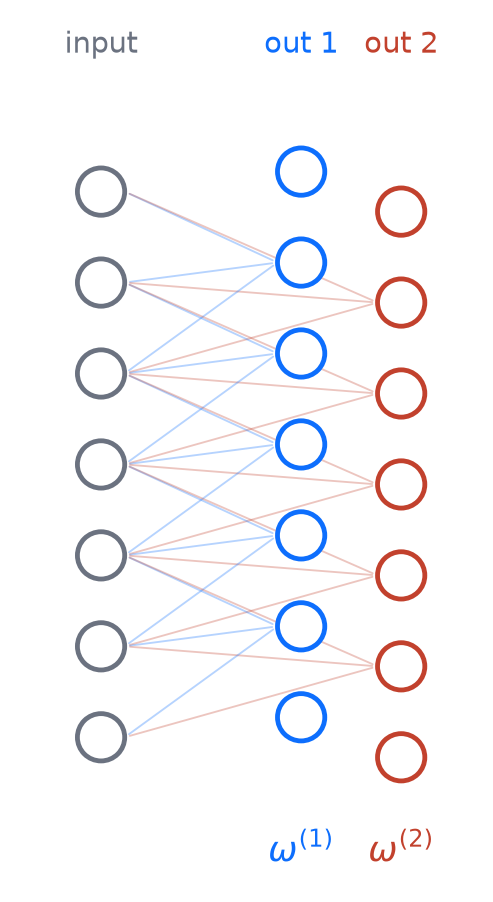
A constrained fully connected layer

Six inputs, six hidden units: 36 independent weights.

The same weighted sum of three neighbours at every position.

Banded weights, tied across positions.

A fully connected layer can reproduce the convolution exactly: set most weights to zero and constrain the rest to be equal. The convolutional layer is the special case, and the constraint is what buys the inductive bias.

Channels

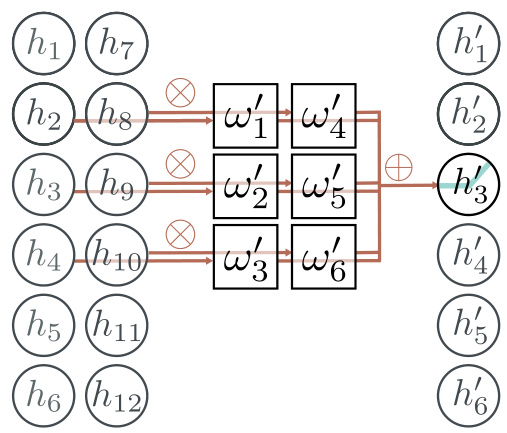
One convolution loses information: neighbours are averaged, and the ReLU clips what falls below zero.

• Several kernels are run in parallel on the same input
• Each produces one set of hidden units — a feature map, or channel
• Each has its own weights and its own bias

Width is recovered in the channel dimension, not the spatial one.

Input channels and output channels

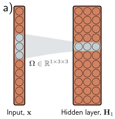
Many in, one out

One kernel per input channel; the responses are summed into a single output channel.

Many out, one in

Repeat with different weights, once per output channel.

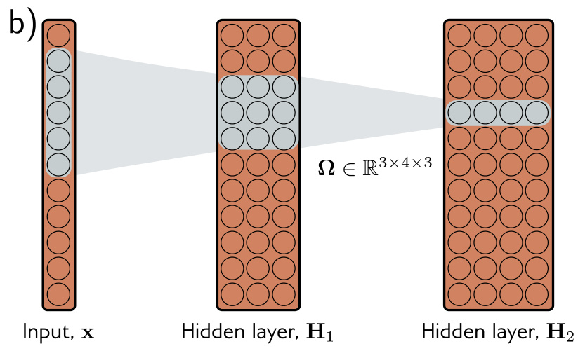
\(C_i\) in, \(C_o\) out

\[\boldsymbol{\Omega} \in \mathbb{R}^{C_i \times C_o \times K}, \quad \boldsymbol{\beta} \in \mathbb{R}^{C_o}\]

Each output unit is a weighted sum over all \(C_i\) channels at \(K\) positions.

No count here depends on the spatial size of the input.

Multiple input channels

One convolution combines both input channels at the three closest positions.

Multiple output channels

• One input channel, two kernels
• Each kernel sweeps every position, with its own weights and bias
• Each produces one output channel
• \(C_o\) channels cost \(C_o\) kernels — the spatial size is untouched

Output channels are parallel readings of the same input.

\(C_i\) in, \(C_o\) out, in matrix form

At each position \(i\), stack the \(K\) neighbouring columns of \(\mathbf{X} \in \mathbb{R}^{C_i \times D}\) into one patch vector:

\[\mathbf{x}_i = \operatorname{vec}\big[\mathbf{X}_{:,\, i-\lfloor K/2\rfloor \,:\, i+\lfloor K/2\rfloor}\big] \in \mathbb{R}^{C_i K}\]

One matrix, one bias, reused at every position:

\[\mathbf{f}_i = \mathbf{a}\big[\boldsymbol{\beta} + \boldsymbol{\Omega}\,\mathbf{x}_i\big], \qquad \boldsymbol{\Omega} \in \mathbb{R}^{C_o \times C_i K}, \quad \boldsymbol{\beta} \in \mathbb{R}^{C_o}\]

\[\mathbf{F} = \big[\,\mathbf{f}_1\;\mathbf{f}_2\;\cdots\;\mathbf{f}_D\,\big] \in \mathbb{R}^{C_o \times D}\]

A convolution is one matrix–vector product per position, with the matrix held fixed.

Written by index, the same statement is \(F_{c,i} = a[\beta_c + \sum_{c'=1}^{C_i}\sum_{k=1}^{K}\Omega_{c,c',k}\,X_{c',\,i+k-\lceil K/2\rceil}]\). The matrix form is what a framework actually computes: the patches are gathered into one matrix and the whole layer becomes a single matrix multiplication.

Receptive fields

The receptive field of a unit \(h^{(k)}_i\) is the set of input positions it depends on:

\[\mathcal{R}\big[h^{(k)}_i\big] = \left\{\, j \;:\; \frac{\partial h^{(k)}_i}{\partial x_j} \neq 0 \,\right\}\]

• Kernel size three, stride one: \(|\mathcal{R}| = 3\), then \(5\), then \(7\)
• A fourth layer covers an eleven-dimensional input entirely

A local operator becomes global by being stacked.

Receptive fields grow with depth

First-layer units cover three input positions.

Second-layer units combine three of those, covering five.

Depth buys context; the parameter count per layer does not change.

Convolutional against fully connected

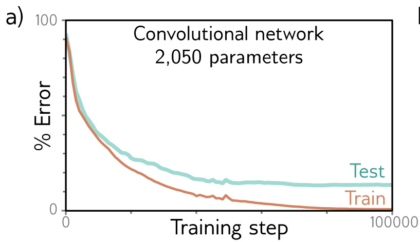
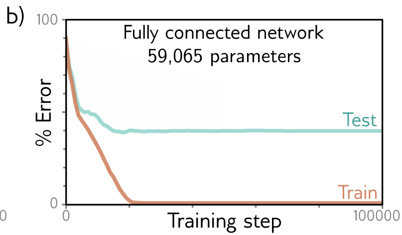
MNIST-1D: a 40D input, ten classes, three hidden layers of fifteen channels.

Convolutional: 2,050 parameters, about 17% test error.

Fully connected: 59,065 parameters, about 40% test error.

Why the gap is not capacity

• Both models fit the training data perfectly
• The fully connected model can represent the other, and does not find it
• Overparameterization usually helps, so the parameter count is not the explanation

What remains is the inductive bias: every position is processed alike, and the data were built by translating a template.

The architecture forbids most of what the other model can say.

Convolution in two dimensions

The 2D operation

The kernel gains a second index and is translated along both axes:

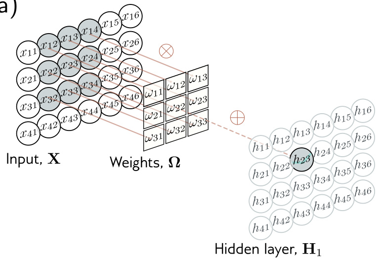
\[h_{ij} = \mathrm{a}\Big[\beta + \sum_{m=1}^{3}\sum_{n=1}^{3} \omega_{mn}\, x_{i+m-2,\, j+n-2}\Big]\]

• A single kernel is now \(K \times K\)
• Padding, stride, dilation carry over, applied one axis at a time

Translating the kernel in two dimensions

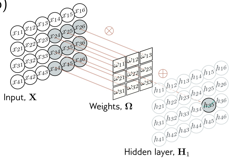
\(h_{23}\) is a weighted sum of the nine positions \(x_{12}\) to \(x_{34}\).

Other outputs come from translating the same kernel.

Channels in two dimensions

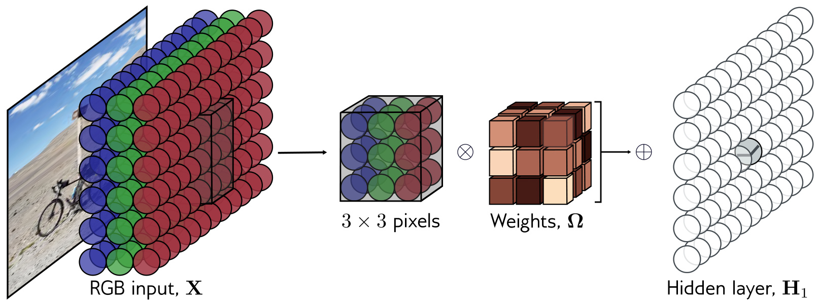
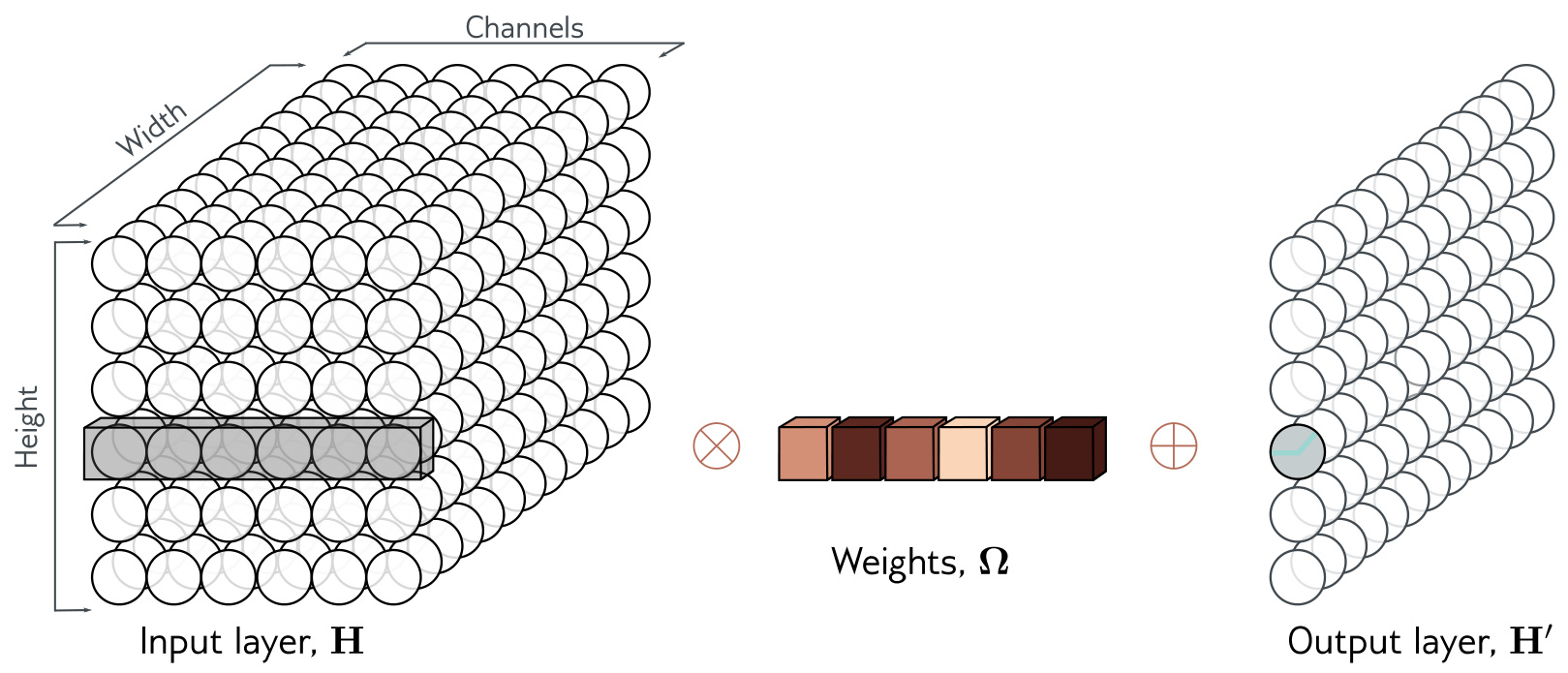
• An RGB image is a 2D signal with three channels
• A \(3\times3\) kernel therefore holds \(3\times3\times3\) weights
• \(C_o\) output channels need \(C_i \times C_o \times K \times K\) weights and \(C_o\) biases

The hidden layer is a tensor: height, width, channels.

Downsampling

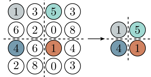
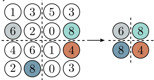
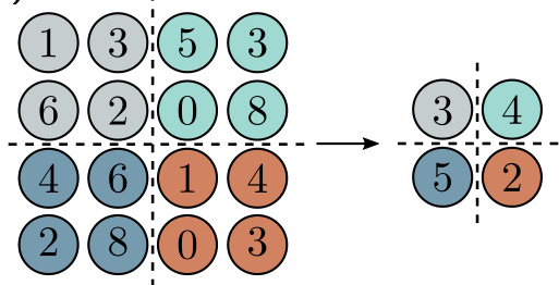
The output of a convolution is a feature map; pooling aggregates non-overlapping regions of it.

Sub-sampling: keep every other position.

Max pooling: the maximum of each \(2\times2\) block.

Mean pooling: the average of each block.

Applied per channel: half the height and width, the same channel count.

Max pooling is where a classifier’s partial translation invariance comes from: shift the input by one pixel and many of the per-block maxima are unchanged. A stride-two convolution achieves sub-sampling at the same time as the convolution, never computing the discarded values.

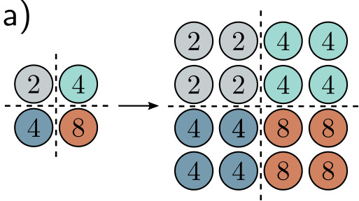
Upsampling without parameters

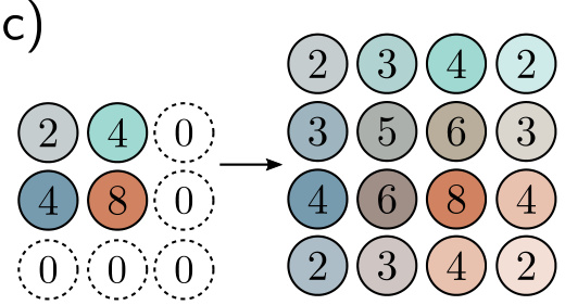
Duplication: each value copied four times.

Max unpooling: values returned to where the maxima came from.

Bilinear interpolation: fill between known samples.

Max unpooling requires the positions recorded by an earlier max pooling layer.

Upsampling with parameters

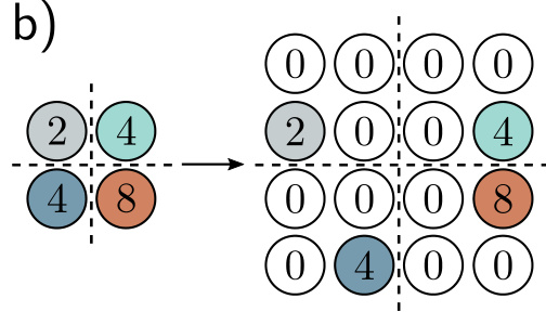
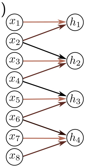
Stride two down: one output per three inputs.

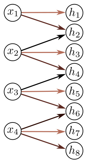
Transposed convolution: one input, three of twice as many outputs.

Its weight matrix is the transpose of the downsampling one.

Changing channels only

• Each output is a weighted sum of all channels at one position
• Weights of size \(1\times1\times C_i \times C_o\) — the 1×1 convolution
• Equivalently: one fully connected network, run at every position

Channel depth and spatial resolution are adjusted independently.

The architectural pattern

A typical convolutional network alternates convolution with downsampling by a factor of two.

• Spatial dimensions fall by factors of two
• Channel counts rise by factors of two
• Fully connected layers at the end integrate across the whole input
• If the output is itself an image, a mirrored decoder upsamples back

Geometry is progressively exchanged for channel depth.

Vision tasks and their architectures

The benchmark

ImageNet — 1,281,167 training images, 1000 categories, a \(224 \times 224\) RGB input.

• The output is a distribution over the 1000 classes
• In 2011, before deep networks: about 25% top-five error

The task that made the case for convolutional architectures.

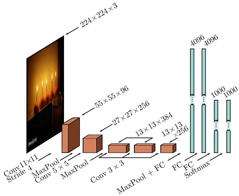
AlexNet

• Eight hidden layers: five convolutional, three fully connected
• \(11\times11\) kernel at stride four, then max pooling, then \(5\times5\) and three \(3\times3\)
• \(6\times6\times256\) reshaped to 9,216, then 4096, 4096, 1000 and a softmax
• About 60 million parameters, most in the fully connected layers

16.4% top-five error, against 25% the year before.

Trained with SGD at momentum 0.9 and batch size 128, dropout in the fully connected layers, an L2 weight-decay regularizer, and a dataset augmented by a factor of 2048. Top-one error was 38.1%.

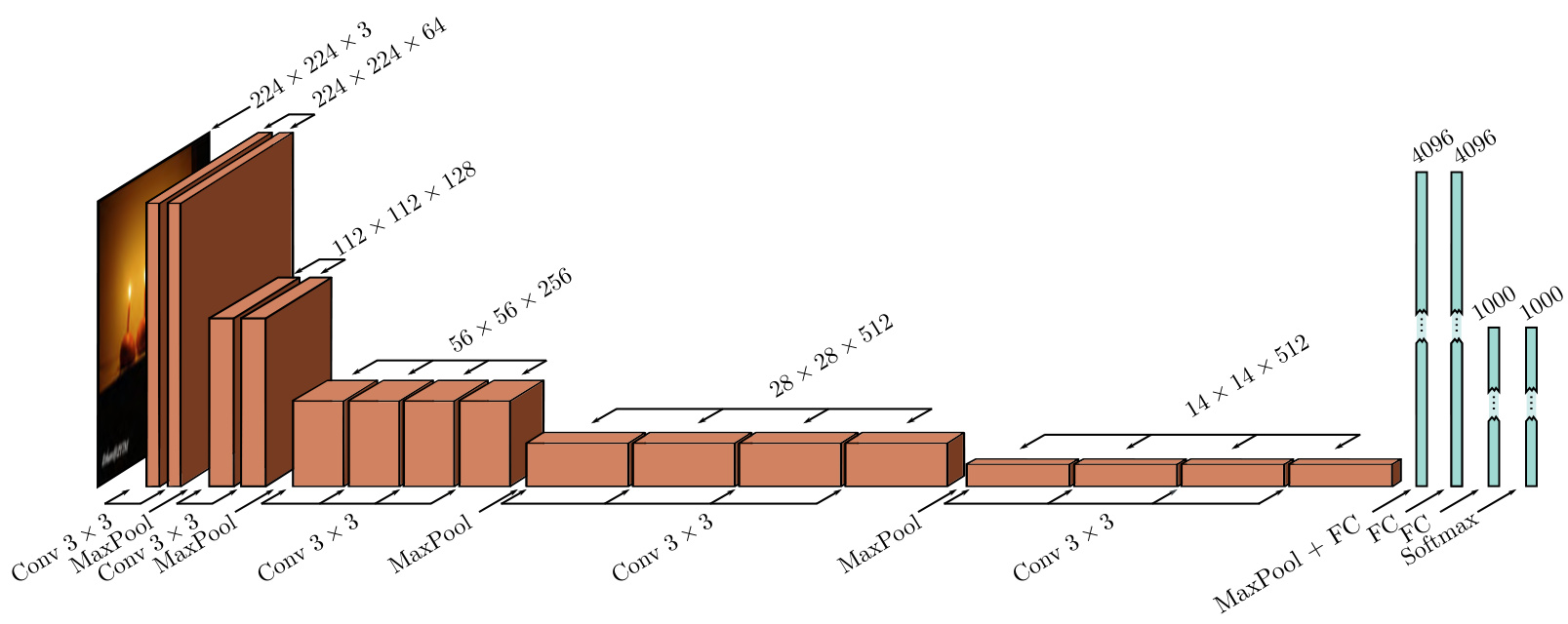
VGG

• The same alternation of convolution and max pooling
• Spatial size falls, channel count rises
• 19 hidden layers, 144 million parameters

6.8% top-five error. The decisive change from AlexNet was depth.

Object detection: YOLO

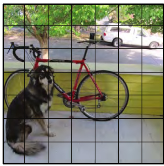
A \(7\times7\) grid, one class per cell.

• A \(448\times448\) input, 24 convolutional layers, VGG-like
• The final \(7\times7\times1024\) map is reshaped, then two fully connected layers
• Each cell predicts a class and a fixed number of boxes
• Five numbers per box: centre \(x\), centre \(y\), height, width, confidence

One pass, then a cleanup

• Low-confidence rectangles are discarded
• Boxes for the same object are suppressed but for the most confident
• The network itself runs once — hence you only look once

Confidence estimates the overlap between the predicted and the ground truth box. The network is pre-trained on ImageNet classification and fine-tuned for detection, with momentum, weight decay, dropout and augmentation.

Semantic segmentation

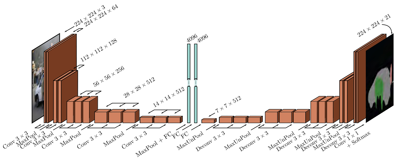
A VGG-derived encoder down to \(14\times14\), a fully connected bottleneck reformed to \(7\times7\times512\), and a mirrored decoder to \(224\times224\times21\).

The encoder-decoder shape

Encoder

• Thirteen convolutional layers, VGG-like
• Downsamples until the receptive field spans the image

Decoder

• Max unpooling and deconvolution layers
• A final \(1\times1\) convolution makes 21 channels, softmax at each position

Also termed an hourglass network, for its shape.

What the bottleneck costs

• The middle representation is low resolution
• Its receptive fields are large, which is what integrates context
• The detail needed for an accurate boundary must survive the bottleneck

Classification improved as networks got deeper — but only up to a point.

Past a certain depth, a plain sequential network becomes difficult to train. The mechanisms that fix it — residual connections and batch normalization — are the subject of the next part of this unit.

The limits of sequential depth

Sequential processing

Every network so far passes each layer’s output to the next, and nothing else:

\[\mathbf{h}_1 = \mathbf{f}_1[\mathbf{x}], \quad \mathbf{h}_2 = \mathbf{f}_2[\mathbf{h}_1], \quad \mathbf{h}_3 = \mathbf{f}_3[\mathbf{h}_2], \quad \mathbf{y} = \mathbf{f}_4[\mathbf{h}_3]\]

Equivalently, one chain of nested functions:

\[\mathbf{y} = \mathbf{f}_4\big[\mathbf{f}_3\big[\mathbf{f}_2[\mathbf{f}_1[\mathbf{x}]]\big]\big]\]

Depth helped from AlexNet to VGG. It does not keep helping.

Deeper stops working

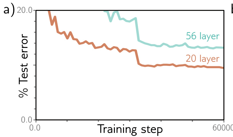
CIFAR-10 test error: 20 layers beat 56.

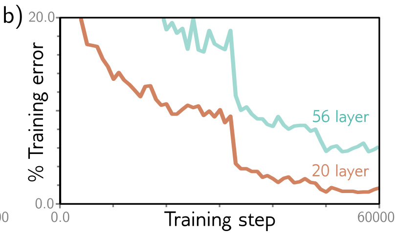
Training error: the same ordering.

Worse on the data it was fitted to — a failure of optimization, not of generalization.

This is the diagnostic that matters. If only the test error had risen, the reading would be overfitting and the response would be regularization. Both rising means the deeper model never found its minimum.

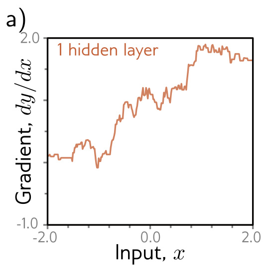
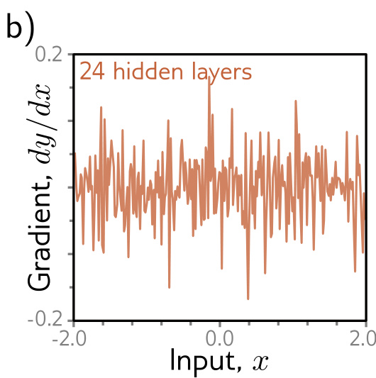
Why: shattered gradients

One hidden layer: \(\partial y/\partial x\) changes slowly with the input.

Twenty-four layers: a tiny change gives a completely different gradient.

The gradient is correct. It is correct only infinitesimally.

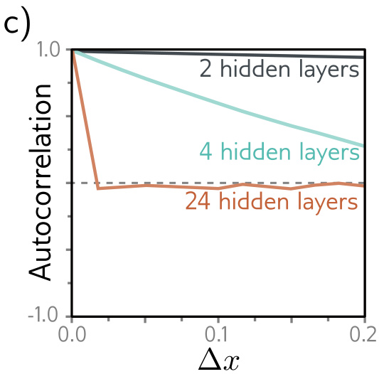
The gradient loses its memory

Autocorrelation of the gradient against depth.

• Nearby gradients are correlated in a shallow network
• The correlation falls to zero as depth grows
• A finite step lands somewhere with an unrelated gradient
• The surface reads as a range of tiny mountains, not one basin

Shattered gradients — the named failure.

Where the shattering comes from

The derivative of the output with respect to the first layer is a product along the chain:

\[\frac{\partial \mathbf{y}}{\partial \mathbf{f}_1} = \frac{\partial \mathbf{f}_2}{\partial \mathbf{f}_1}\frac{\partial \mathbf{f}_3}{\partial \mathbf{f}_2}\frac{\partial \mathbf{f}_4}{\partial \mathbf{f}_3}\]

• Change \(\boldsymbol{\phi}_1\) and every factor is evaluated somewhere else
• Because \(\mathbf{f}_2, \mathbf{f}_3, \mathbf{f}_4\) are themselves computed from \(\mathbf{f}_1\)
• The longer the chain, the less the new product resembles the old

Residual connections

The definition

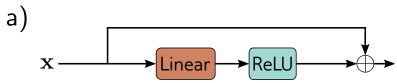
A residual, or skip, connection adds each layer’s input back to its output:

\[\mathbf{h}_k = \mathbf{h}_{k-1} + \mathbf{f}_k\big[\mathbf{h}_{k-1}, \boldsymbol{\phi}_k\big]\]

• Each \(\mathbf{f}_k\) learns an additive change to the current representation
• So its output must be the same shape as its input
• The combination is a residual block

The branch learns a correction to the identity, not a replacement for it.

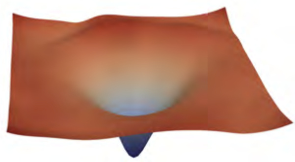
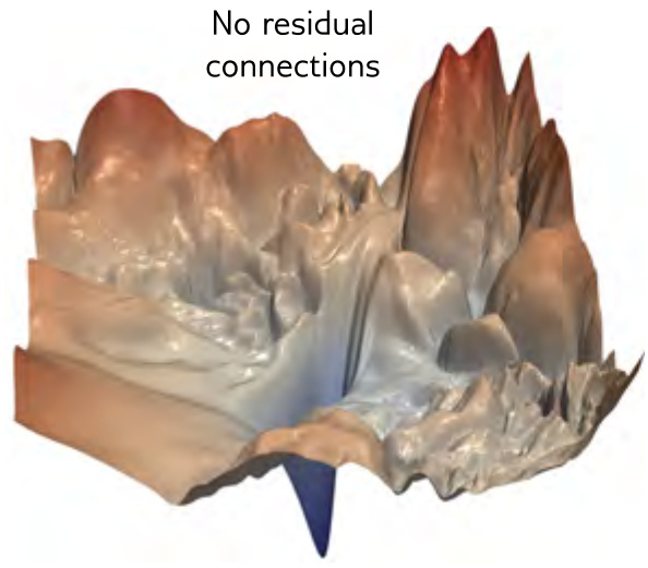
What it does to the loss surface

56 layers, with skip connections.

The same network, skips removed.

One addition per block, and the surface becomes descendable.

Both surfaces are plotted in two random parameter directions around the minimum found by SGD on CIFAR-10, with the directions normalized so the comparison is fair.

Unraveling

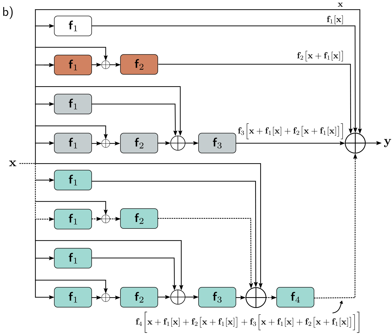
\[\mathbf{y} = \mathbf{x} + \mathbf{f}_1[\mathbf{x}] + \mathbf{f}_2\big[\mathbf{x}+\mathbf{f}_1[\mathbf{x}]\big] + \cdots\]

• The output is the input plus four smaller networks
• Equivalently, sixteen paths of differing length
• An ensemble, summed

The identity term

Eight of the sixteen paths contain \(\mathbf{f}_1\), one of length one:

\[\frac{\partial \mathbf{y}}{\partial \mathbf{f}_1} = \mathbf{I} + \frac{\partial \mathbf{f}_2}{\partial \mathbf{f}_1} + \Big(\frac{\partial \mathbf{f}_3}{\partial \mathbf{f}_1} + \frac{\partial \mathbf{f}_2}{\partial \mathbf{f}_1}\frac{\partial \mathbf{f}_3}{\partial \mathbf{f}_2}\Big) + \cdots\]

• A sum of paths, where the sequential network had one product
• \(\mathbf{I}\) is a direct route from every layer to the output

Gradients no longer have to survive the whole chain.

Order of operations

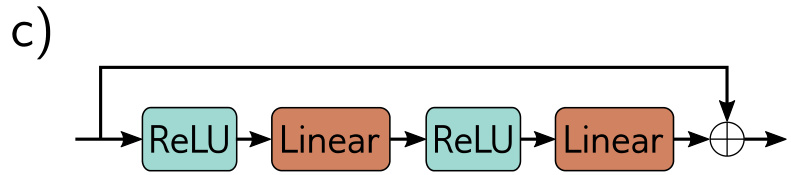
Linear then ReLU — the block’s output is non-negative, so it can only add.

ReLU then linear — both signs available.

The block must stay nonlinear, or the whole network collapses to a linear map.

A block that begins with a ReLU does nothing at all if the network input is negative, since the ReLU clips the entire signal; networks therefore start with a linear transformation rather than with a residual block.

Several layers to a block

• A block may hold several layers of processing
• It usually terminates in a linear transformation
• Residual links roughly double the trainable depth

Beyond that, the variance of the forward pass has to be managed.

Batch normalization

The variance doubles at every block

1, 2, 4, 8 — exponential in the number of blocks.

• The block preserves variance, and the input carries its own
• The two branches are uncorrelated, so variance adds
• Floating point precision is exceeded before the network is deep

Two ways to stop it

Rescale by \(1/\sqrt{2}\) after each block: variance held at one.

BatchNorm first in each block: growth becomes linear, 2, 3, 4.

The second is what is used in practice.

The operation

Per activation \(h\), over the batch \(\mathcal{B}\):

\[m_h = \frac{1}{|\mathcal{B}|}\sum_{i \in \mathcal{B}} h_i, \qquad s_h = \sqrt{\frac{1}{|\mathcal{B}|}\sum_{i \in \mathcal{B}} (h_i - m_h)^2}\]

Standardize, then apply a learned scale and offset:

\[h_i \leftarrow \frac{h_i - m_h}{s_h + \epsilon}, \qquad h_i \leftarrow \gamma h_i + \delta\]

Mean \(\delta\) and standard deviation \(\gamma\), both learned like any other parameter.

Applied independently to each hidden unit. In a convolutional network the statistics are taken over the batch and the spatial positions together, so \(K\) layers of \(C\) channels carry \(KC\) scales and \(KC\) offsets.

Training and inference differ

At test time there is no batch to take statistics from.

• \(m_h\) and \(s_h\) are recomputed over the whole training set and frozen
• The deployed network is therefore not the same function as the one trained

A rare case where the model at test time is not the model that was fitted.

What it costs, and what it buys

The cost

• Two parameters, \(\gamma\) and \(\delta\), at every hidden unit
• Rescaling the weights changes nothing, so the weights are redundant

The benefit

• Stable forward pass — variance grows linearly, not exponentially
• Higher learning rates — a smoother, more predictable surface
• Regularization — batch statistics inject noise

At initialization the later layers change the overall variation less than the earlier ones, so the network is effectively shallower at the start of training and can increase the scales in later layers to control its own effective depth.

Residual architectures in practice

ResNet

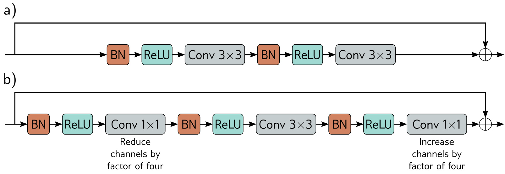
Standard block

BatchNorm, ReLU, convolution — twice, then added back.

Bottleneck block

\(1\times1\) cuts the channels, \(3\times3\) does the spatial work, \(1\times1\) restores them.

The same \(3\times3\) receptive field, at a fraction of the parameters.

ResNet-200 against its predecessors

Network	Layers	Top-5	Top-1
AlexNet	8	16.4%	38.1%
VGG	19	6.8%	23.7%
ResNet-200	200	4.8%	20.1%

Human performance on this task is estimated at 5.1% top-5.

The architecture follows AlexNet and VGG in shape — resolution falls while channels rise — but uses bottleneck blocks throughout, a 7x7 convolution at the front, and a fully connected layer to 1000 classes at the end. Resolution is reduced between blocks by stride-two convolutions.

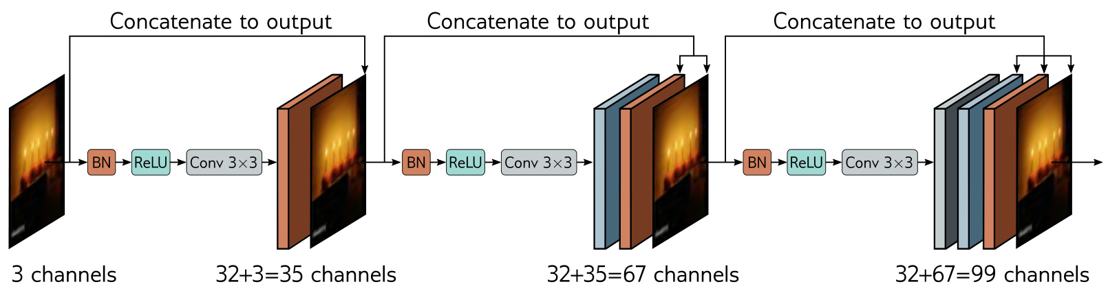
DenseNet

• Concatenate rather than add
• Each layer sees the outputs of all previous layers
• 3 channels → 32 processed → 35 → another 32 → 67 → …
• \(1\times1\) convolutions cut the channel count back

Concatenation cannot cross a downsampling, so each resolution starts a new chain.

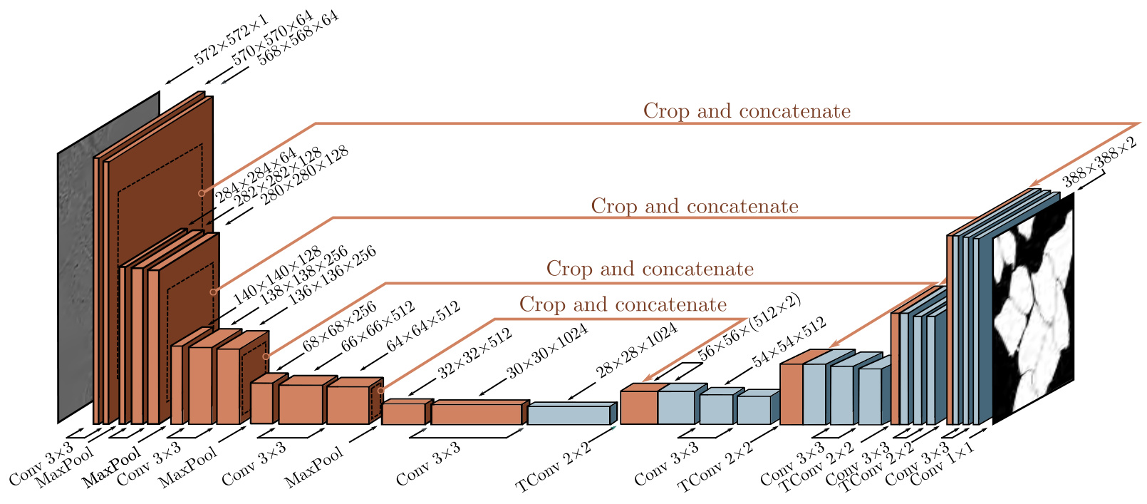
U-Net

• The encoder’s representation is concatenated to the decoder at the matching scale
• The bottleneck no longer has to remember spatial detail
• Fully convolutional, so it runs at any input size

The long skip is the same idea, at the scale of a whole encoder stage.

The original used valid convolutions, so each encoder representation is larger than its decoder partner and must be cropped before concatenation; zero-padded implementations avoid the cropping. Hourglass networks instead apply convolutions inside the skip and add rather than concatenate, and a chain of them — a stacked hourglass — is used for pose estimation, one heatmap per joint.

Why residual networks work

The loss surface account

Explains why the network trains at all: a smooth basin is descendable by a finite step, and its minimum is robust.

The ensemble account

Explains why width can substitute for depth, and why gradients never traverse the longest paths.

Neither account says the depth itself is responsible — a plain 56-layer network trains worse.

Summary

🎯 What this unit established

1. Vision needs equivariance, and convolution builds it in rather than learning it
2. A convolution is a fully connected layer with banded, tied weights — four parameters, not \(D^2\)
3. Depth buys receptive field; channels buy the representation back
4. Past a point, sequential depth stops training — and residual connections restore it

The inductive bias is the whole of the advantage.

🚀 Where next

The Computer Vision module takes these architectures as its subject rather than its conclusion.

• Early convolutional networks for images, in detail
• Residual convolutional networks
• Object detection, from the early networks to the fast ones

The same kernel, at the scale of a working system. 🔍