---
title: Lecture notes — Preliminaries to Machine Learning
keywords:
- ver. 1.2.2
- preliminaries_to_machine_learning
date: 2026-09-02
---
[← Preliminaries to Machine Learning](index.qmd){.hg-back}
[ver. 1.2.2 · 2026-09-08 16:21:38]{.hg-stamp}
## Where this fits
This is the first unit of *Basics to Machine Learning*. Three prerequisites are used and
no others: the equation of a straight line in terms of its intercept and slope;
matrix–vector multiplication, together with the dimensions that make a product defined;
and the partial derivative, used only to give meaning to the phrase *the gradient of a
surface*.
One template organises the whole unit. It is stated once and never varied:
- a **model** — a family of functions $\mathbf{y} = \mathbf{f}[\mathbf{x}, \boldsymbol{\phi}]$, whose particular member is fixed by the parameters $\boldsymbol{\phi}$;
> The functional form is chosen by the designer. The parameters are not.
- a **loss** — a scalar $L[\boldsymbol{\phi}]$ measuring how badly a given choice of parameters predicts a training set;
> Lower is better, and the loss is the only quantity training consults.
- a **training** procedure — a search for the parameters at which the loss is small.
The three model families treated below are the straight line, the shallow network and
the deep network. They differ in the first item of the template and in nothing else.
## Learning outcomes
1. `frame-supervised-learning` — Frame a prediction task as a supervised learning problem with a parameterized model, a dataset, and a loss.
2. `build-1d-linear-regression` — Build the 1D linear regression model and write its least-squares loss.
3. `evaluate-generalization` — Distinguish training error from test error and diagnose underfitting versus overfitting.
4. `construct-shallow-network` — Construct a shallow ReLU network and trace how it produces a piecewise linear function.
5. `apply-universal-approximation` — State the universal approximation theorem and say what it does and does not promise.
6. `generalize-multivariate` — Extend a shallow network to multivariate inputs and outputs and count its parameters.
7. `compose-into-deep-networks` — Compose layers into a deep network and explain how folding multiplies linear regions.
8. `write-matrix-form` — Write a $K$-layer network in matrix notation and name its hyperparameters.
9. `compare-depth-and-width` — Compare deep and shallow networks on expressivity per parameter and on practical trainability.
## Concepts introduced
- **Supervised learning** — a mapping from inputs to outputs, learned from paired examples.
- **Inference** — computing a prediction by evaluating the model equation at a given input.
- **Loss function** — a scalar measure of the mismatch between predictions and training targets.
- **Linear regression** — the straight-line model $y = \phi_0 + \phi_1 x$, parameterized by intercept and slope.
- **Model training** — the search for the parameters at which the loss is minimal.
- **Generalization and testing** — measuring performance on data held out from training.
- **Underfitting and overfitting** — the two failure modes of a mismatched model capacity.
- **Shallow neural network** — a network with one hidden layer between input and output.
- **Rectified linear unit** — the activation $a[z] = \max(0, z)$, which clips negative values to zero.
- **Pre-activations and activations** — the values entering and the values leaving the activation function.
- **Linear regions and joints** — the pieces into which a ReLU network divides its input space, and the boundaries between them.
- **Network capacity** — the total number of hidden units.
- **Universal approximation theorem** — an existence result: sufficient width suffices for arbitrary accuracy.
- **Deep neural network** — a network with more than one hidden layer.
- **Folding input space** — the geometric reading of composition, in which one layer maps distinct inputs to the same intermediate value.
- **Hyperparameters** — depth and width, chosen before the parameters are learned.
- **Matrix formulation** — each layer computed as $\mathbf{h}_{k} = \mathbf{a}[\boldsymbol{\beta}_{k-1} + \boldsymbol{\Omega}_{k-1}\mathbf{h}_{k-1}]$.
- **Depth efficiency** — the property that certain functions are exponentially cheaper for a deep network than for a shallow one.
## The supervised learning framework
A **supervised learning model** defines a mapping from one or more inputs to one or more
outputs. The worked case in *Understanding Deep Learning* is the valuation of a
second-hand car: the input is the car's age and mileage, the output is its estimated
value in dollars.
Both input and output are assumed to be vectors of predetermined, fixed size whose
elements always appear in the same order — age first, then mileage, in every example.
Data of this form is termed **structured** or **tabular** data. The model is a function
$\mathbf{f}[\bullet]$ taking $\mathbf{x}$ and returning $\mathbf{y}$:
$$\mathbf{y} = \mathbf{f}[\mathbf{x}].$$
Computing the prediction $\mathbf{y}$ from the input $\mathbf{x}$ is termed
**inference**. The model is a mathematical equation of fixed form containing
**parameters** $\boldsymbol{\phi}$, and the choice of parameters determines which
particular input–output relation the equation expresses. The honest form of the model
therefore carries the parameters explicitly:
$$\mathbf{y} = \mathbf{f}[\mathbf{x}, \boldsymbol{\phi}].$$
The equation names a family of relations; the parameters name one member of that family.
**Learning** or **training** a model means finding parameters that produce sensible
predictions. The parameters are learned from a **training dataset** of $I$ pairs of
input and output examples $\{\mathbf{x}_i, \mathbf{y}_i\}$. The degree of mismatch in
this mapping is quantified by the **loss** $L$, a single scalar summarising how poorly
the model with parameters $\boldsymbol{\phi}$ predicts the training outputs from the
training inputs. Treated as a function of the parameters, the loss becomes the objective
of a minimization:
$$\hat{\boldsymbol{\phi}} = \operatorname*{argmin}_{\boldsymbol{\phi}}\Big[L[\boldsymbol{\phi}]\Big].$$
Two features of this formulation are easily missed.
- The loss depends on the training data as well as on the parameters.
> Written in full it is $L[\{\mathbf{x}_i, \mathbf{y}_i\}, \boldsymbol{\phi}]$. The data are suppressed from the notation because they are held fixed while $\boldsymbol{\phi}$ varies, not because they are absent.
- A small loss after minimization establishes only that the model predicts the *training* outputs accurately.
> Performance is afterwards assessed on separate **test data**, to determine how well the model **generalizes** to examples it did not observe during training. Only if that performance is adequate is the model ready for deployment.
Inference is a single evaluation of the function with the parameters held fixed, and is
computationally inexpensive. Training searches the space of parameters for the value
minimizing the loss. [The asymmetry between one evaluation and a search over a parameter
space]{.hg-key} holds for every model treated in this unit.
::: {.column-margin}
Strictly, a *loss function* is the term associated with a single data point, a *cost
function* is the overall quantity minimized, and an *objective function* is any function
to be maximized or minimized. The first two are used interchangeably in most of the
literature and in these notes.
:::
::: {.callout-note title="Discriminative and generative formulations"}
A model of the form $\mathbf{y} = \mathbf{f}[\mathbf{x}, \boldsymbol{\phi}]$ is
**discriminative**: it predicts the output directly from the measurement. The alternative
is a **generative** model $\mathbf{x} = \mathbf{g}[\mathbf{y}, \boldsymbol{\phi}]$, which
computes the measurement as a function of the output, and into which prior knowledge —
of 3D geometry or of optics, say — can be built. Inference then requires inverting the
generative equation as $\mathbf{y} = \mathbf{g}^{-1}[\mathbf{x}, \boldsymbol{\phi}]$,
which may be difficult. Discriminative models dominate modern practice: the advantage of
built-in prior knowledge is usually outweighed by fitting very flexible discriminative
models to large quantities of training data.
:::
::: {.callout-note collapse="true" title="Outcomes and concepts"}
**Learning outcomes**
- {{< badge outcome "frame-supervised-learning" >}} Frame a prediction task as a supervised learning problem with a parameterized model, a dataset, and a loss.
**Concepts**
- {{< badge concept "supervised-learning" >}} a parameterized function $\mathbf{y} = \mathbf{f}[\mathbf{x}, \boldsymbol{\phi}]$ is fitted to training pairs $\{\mathbf{x}_i, \mathbf{y}_i\}$ so that it predicts outputs for new inputs
- {{< badge concept "inference" >}} evaluating the model equation at an input, with the parameters already fixed, produces a prediction
- {{< badge concept "loss-function" >}} a scalar $L[\boldsymbol{\phi}]$ measures the mismatch between the model's predictions and the training targets
- {{< badge concept "model-training" >}} training is the minimization $\hat{\boldsymbol{\phi}} = \operatorname{argmin}_{\boldsymbol{\phi}} L[\boldsymbol{\phi}]$ over the training examples
- {{< badge concept "generalization-and-testing" >}} performance is measured on separate test data before deployment, since the training loss alone does not establish it
:::
## Linear regression and its loss surface
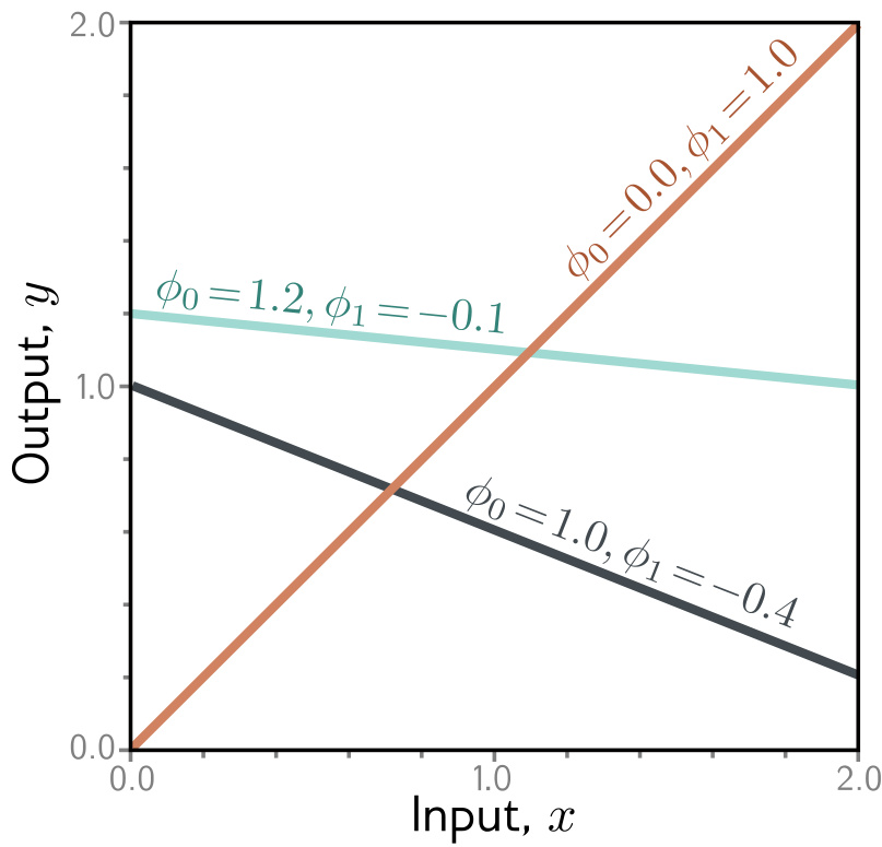
A **1D linear regression** model describes the relationship between a scalar input $x$
and a scalar output $y$ as a straight line:
$$y = \mathrm{f}[x, \boldsymbol{\phi}] = \phi_0 + \phi_1 x.$$
The model has two parameters, $\boldsymbol{\phi} = [\phi_0, \phi_1]$, where $\phi_0$ is
the y-intercept of the line and $\phi_1$ is its slope. Different choices of intercept and
slope give different relations between input and output. The equation defines the family
of all lines; the parameters select the particular line.
### The least-squares loss
Choosing among candidate lines requires a numerical criterion. The **loss** assigns to
each choice of parameters a value quantifying the mismatch between model and data; a
lower loss means a better fit.
The mismatch at example $i$ is the deviation between the model's prediction
$\mathrm{f}[x_i, \boldsymbol{\phi}]$ — the height of the line at $x_i$ — and the observed
output $y_i$. The total mismatch, termed the **training error** or the loss, is the sum
of the squares of these deviations over all $I$ training pairs:
$$L[\boldsymbol{\phi}] \;=\; \sum_{i=1}^{I}\big(\mathrm{f}[x_i, \boldsymbol{\phi}] - y_i\big)^2 \;=\; \sum_{i=1}^{I}\big(\phi_0 + \phi_1 x_i - y_i\big)^2.$$
Because the best parameters minimize this expression, it is termed a **least-squares**
loss. The squaring makes the direction of the deviation immaterial: a point lying above
the line is penalised exactly as much as a point the same distance below it. A
probabilistic justification for this particular choice exists, and is the subject of the
next unit.
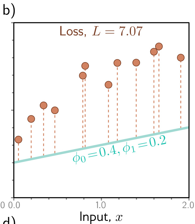
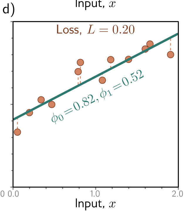
On a dataset of $I = 12$ points, the difference between poor and good parameters is a
difference of nearly two orders of magnitude in the loss. The lines $\phi_0 = 0.4,
\phi_1 = 0.2$ and $\phi_0 = 1.60, \phi_1 = -0.8$ give losses of $L = 7.07$ and
$L = 10.28$; the best-fitting line, $\phi_0 = 0.82, \phi_1 = 0.52$, gives $L = 0.20$,
the smallest loss attainable by any line on this data.
:::: {.columns}
::: {.column width="48%"}
:::
::: {.column width="48%"}
:::
::::
### The loss as a surface
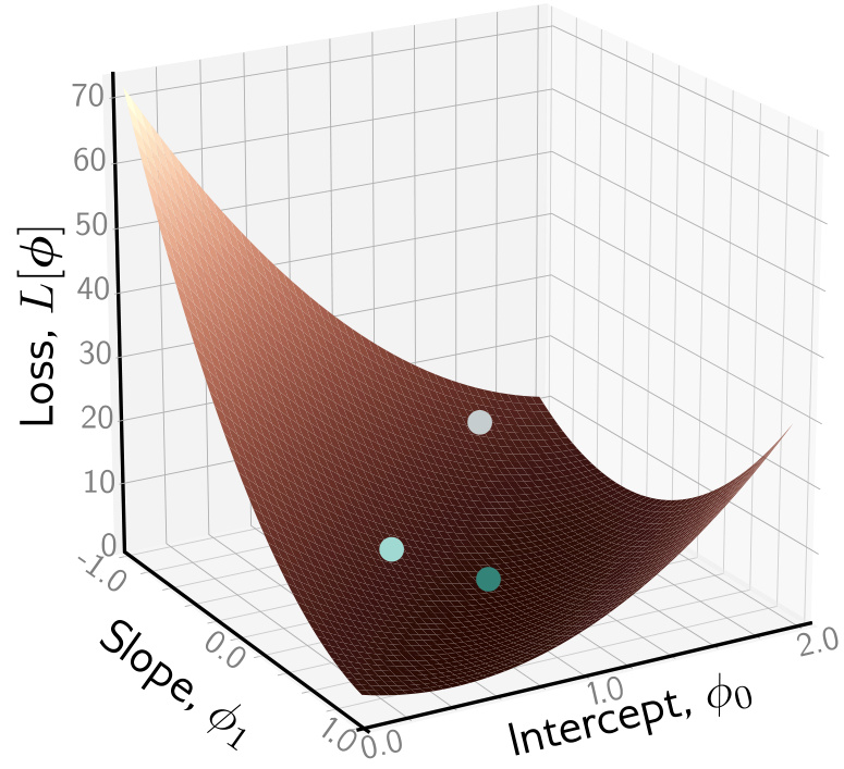
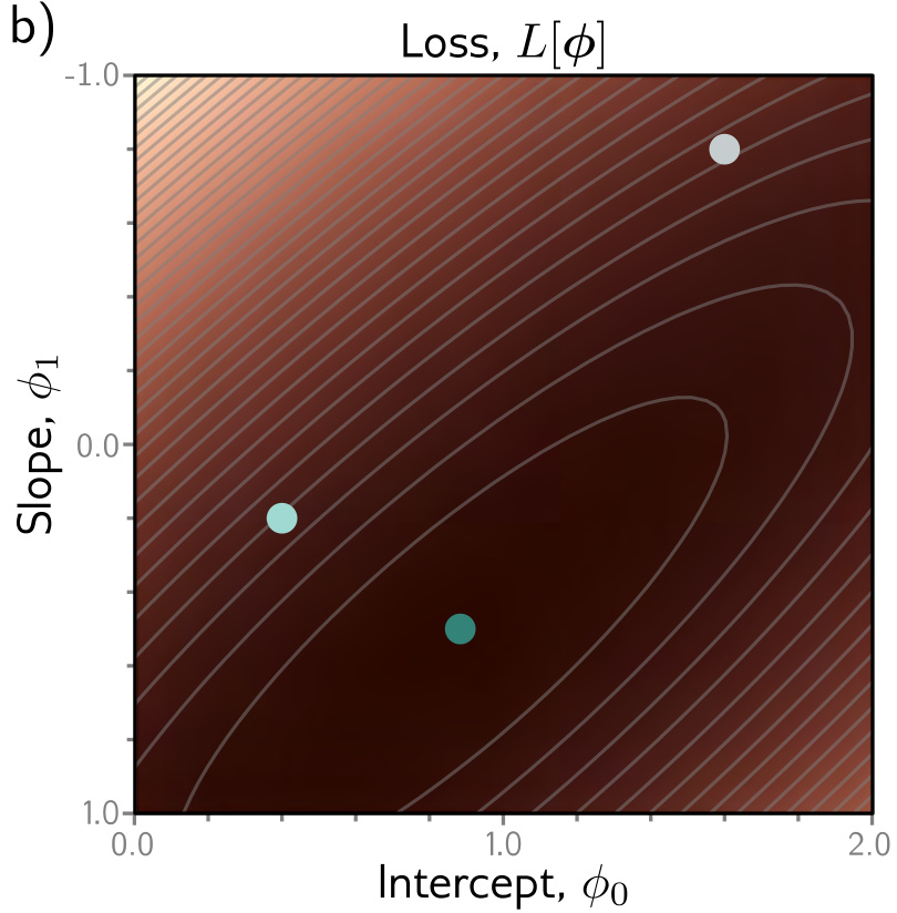
With only two parameters, the loss can be evaluated for every combination of intercept
and slope and displayed in full. The result is a surface over the parameter space: a
bowl whose height above the point $(\phi_0, \phi_1)$ is the loss of the corresponding
line. Viewed from above, the same object becomes a heatmap with elliptical isocontours.
:::: {.columns}
::: {.column width="48%"}
![The loss $L[\boldsymbol{\phi}]$ as a surface over intercept and slope.](chapter_2_supervised_learning/img-5.jpeg)
:::
::: {.column width="48%"}
:::
::::
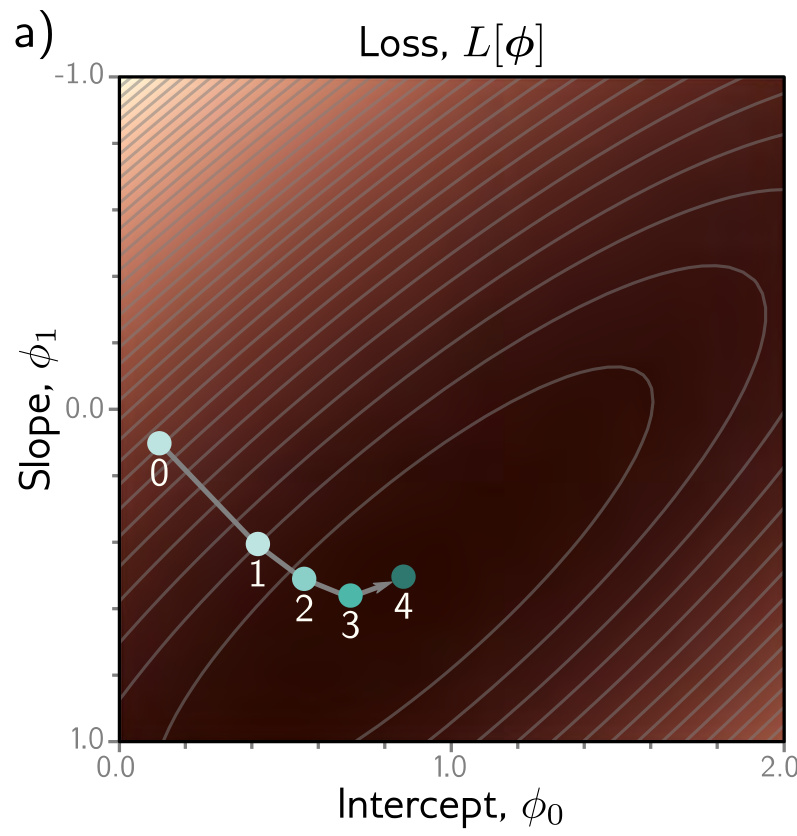
The surface is the object training searches. Finding the parameters that minimize the
loss is termed **model fitting**, **training**, or **learning**, and the basic method is
to choose the initial parameters at random and then improve them by walking down the loss
function until the bottom is reached. One way to do so is to measure the gradient of the
surface at the current position and take a step in the most steeply downhill direction,
repeating until the gradient is flat and no further improvement can be made.
::: {.callout-important title="The iterative method is not needed here — and that is the point"}
For linear regression under a least-squares loss, the partial derivatives $\partial
L/\partial\phi_0$ and $\partial L/\partial\phi_1$ can be set to zero and solved, yielding
the optimal parameters in closed form. The descent procedure is introduced not because
this model requires it, but because it continues to work for more complex models where no
closed-form solution exists and where there are far too many parameters to evaluate the
loss for every combination of values.
:::
::: {.callout-note collapse="true" title="Outcomes and concepts"}
**Learning outcomes**
- {{< badge outcome "build-1d-linear-regression" >}} Build the 1D linear regression model and write its least-squares loss.
- {{< badge outcome "frame-supervised-learning" >}} Frame a prediction task as a supervised learning problem with a parameterized model, a dataset, and a loss.
**Concepts**
- {{< badge concept "linear-regression" >}} the straight line $y = \phi_0 + \phi_1 x$ is a two-parameter family whose members are selected by an intercept and a slope
- {{< badge concept "loss-function" >}} the least-squares loss $L[\boldsymbol{\phi}] = \sum_i (\phi_0 + \phi_1 x_i - y_i)^2$ is a surface over the two-dimensional parameter space
- {{< badge concept "model-training" >}} parameters are improved from a random start by repeatedly stepping in the steepest downhill direction on that surface
- {{< badge concept "supervised-learning" >}} the general framework becomes concrete and drawable when the model has one input, one output and two parameters
:::
## Testing and generalization
The loss attained after training measures performance on the training data alone. The
quantity of interest is performance in the real world, and it is obtained by computing
the loss on a separate set of **test data**. The degree to which prediction accuracy
**generalizes** to the test data depends in part on how representative and how complete
the training data is. It also depends on the model.
Two failure modes are distinguished, and they are opposites.
- **Underfitting** — the model family is too restrictive to capture the true relationship between input and output.
> A straight line fitted to data that curves is the standard case. No choice of intercept and slope reduces the training loss much, and the test loss is correspondingly poor. The deficiency lies in the family, not in the search.
- **Overfitting** — a very expressive model describes statistical peculiarities of the training data that are atypical, and makes unusual predictions as a result.
> Here the training loss can be driven very low precisely because the model has enough capacity to accommodate the noise in the particular sample. The training loss is then no longer evidence of anything.
The two modes are the reason model **capacity** — for a neural network, the number of
hidden units — is a design decision rather than a quantity to be maximised. The families
introduced in the remainder of this unit are progressively more expressive than the
straight line, and each step buys the ability to fit more relationships at the cost of a
greater exposure to the second failure mode.
::: {.callout-note title="What the linear regression example has established"}
A supervised learning model is a function $\mathbf{y} = \mathbf{f}[\mathbf{x},
\boldsymbol{\phi}]$ relating inputs to outputs, whose particular relationship is
determined by the parameters $\boldsymbol{\phi}$. To train it, a loss function
$L[\boldsymbol{\phi}]$ is defined over a training dataset $\{\mathbf{x}_i,
\mathbf{y}_i\}$, quantifying the mismatch between the model's predictions and the
observed outputs as a function of the parameters. The parameters minimizing that loss are
then sought. The result is evaluated on a different set of test data to determine how
well it generalizes to new inputs.
The one drawback of 1D linear regression, and the reason the unit continues, is that it
can only describe the relationship between input and output as a straight line.
:::
Shallow neural networks, treated next, are only slightly more complex than linear
regression but describe a much larger family of input–output relations. Deep networks are
just as expressive as shallow ones, and describe complex functions with fewer parameters.
::: {.callout-note collapse="true" title="Outcomes and concepts"}
**Learning outcomes**
- {{< badge outcome "evaluate-generalization" >}} Distinguish training error from test error and diagnose underfitting versus overfitting.
**Concepts**
- {{< badge concept "generalization-and-testing" >}} the loss is recomputed on data held out from training, and that value is what generalization is judged by
- {{< badge concept "underfitting-and-overfitting" >}} an insufficiently expressive family cannot capture the true relationship, while an overly expressive one fits the training sample's noise
- {{< badge concept "linear-regression" >}} the straight-line family is the elementary case of underfitting, since it represents no relationship other than a line
:::
## Shallow networks and piecewise linear functions
A **shallow neural network** is a function $\mathbf{y} = \mathbf{f}[\mathbf{x},
\boldsymbol{\phi}]$ mapping multivariate inputs to multivariate outputs through a single
hidden layer. The mechanism is visible in an example network mapping a scalar input $x$
to a scalar output $y$ with ten parameters $\boldsymbol{\phi} = \{\phi_0, \phi_1, \phi_2,
\phi_3, \theta_{10}, \theta_{11}, \theta_{20}, \theta_{21}, \theta_{30}, \theta_{31}\}$:
$$y = \mathrm{f}[x, \boldsymbol{\phi}] = \phi_0 + \phi_1 a[\theta_{10} + \theta_{11}x] + \phi_2 a[\theta_{20} + \theta_{21}x] + \phi_3 a[\theta_{30} + \theta_{31}x].$$
The calculation breaks into three parts. Three linear functions of the input are computed;
the three results are passed through an **activation function** $a[\bullet]$; the three
activations are weighted by $\phi_1, \phi_2, \phi_3$, summed, and given the offset
$\phi_0$.
The activation function used throughout is the **rectified linear unit**, or **ReLU**:
$$a[z] = \mathrm{ReLU}[z] = \begin{cases} 0 & z < 0 \\ z & z \ge 0. \end{cases}$$
It returns the input when the input is positive, and zero otherwise — it clips negative
values to zero.
### Hidden units and joints
Naming the intermediate quantities makes the structure explicit. The three **hidden
units** are
$$h_1 = a[\theta_{10} + \theta_{11}x], \qquad h_2 = a[\theta_{20} + \theta_{21}x], \qquad h_3 = a[\theta_{30} + \theta_{31}x],$$
and the output is a linear function of them:
$$y = \phi_0 + \phi_1 h_1 + \phi_2 h_2 + \phi_3 h_3.$$
Each hidden unit contains a linear function $\theta_{\bullet 0} + \theta_{\bullet 1}x$ of
the input, clipped below zero by the ReLU. The position at which unit $d$ switches
between clipped and unclipped is the input value where its linear function crosses zero;
solving $\theta_{d0} + \theta_{d1}x = 0$ gives
$$x = -\frac{\theta_{d0}}{\theta_{d1}}.$$
These positions become the **joints** in the final output. Each hidden unit contributes
one joint, so a network with three hidden units produces a continuous piecewise linear
function with up to four **linear regions**.
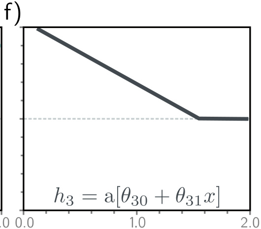
Each linear region corresponds to a different **activation pattern** in the hidden units.
A clipped unit is termed **inactive**; an unclipped unit is termed **active**. The slope
of a region is determined by the slopes $\theta_{\bullet 1}$ of the linear functions that
are active there together with the output weights $\phi_{\bullet}$ subsequently applied to
them. In the shaded region above, where $h_1$ and $h_3$ are active and $h_2$ is not, the
slope is $\theta_{11}\phi_1 + \theta_{31}\phi_3$.
::: {.callout-important title="Three joints, but only three independent slopes"}
Three hidden units give four linear regions, and it is tempting to read that as four
degrees of freedom in the slopes. Only three of the four slopes are independent. The
fourth is either zero — if every hidden unit is inactive in that region — or a sum of the
slopes of the other regions.
:::
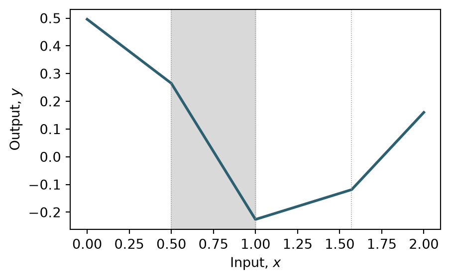
The parameters of the figure above are $\boldsymbol{\phi} = \{-0.23, -1.3, 1.3, 0.66,
-0.2, 0.4, -0.9, 0.9, 1.1, -0.7\}$, in the order listed earlier. The joints therefore lie
at $x = 0.2/0.4 = 0.5$, at $x = 0.9/0.9 = 1.0$, and at $x = 1.1/0.7 \approx 1.57$, and
the slope in the shaded region between the first two is $0.4 \times (-1.3) + (-0.7) \times
0.66 = -0.98$.
```{python}
#| label: fig-shallow-example
#| fig-cap: "The example network evaluated at its stated parameters. The three joints fall at $x = 0.5$, $x = 1.0$ and $x \\approx 1.57$; the segment between the first two has slope $-0.98$."
import numpy as np
import matplotlib.pyplot as plt

phi0, phi1, phi2, phi3 = -0.23, -1.3, 1.3, 0.66
theta = [(-0.2, 0.4), (-0.9, 0.9), (1.1, -0.7)]

x = np.linspace(0.0, 2.0, 1001)
h = [np.maximum(0.0, t0 + t1 * x) for t0, t1 in theta]
y = phi0 + phi1 * h[0] + phi2 * h[1] + phi3 * h[2]

fig, ax = plt.subplots(figsize=(5, 3))
ax.plot(x, y, color="#2c5f70", linewidth=2)
ax.axvspan(0.5, 1.0, color="0.85")
for joint in (0.5, 1.0, 1.1 / 0.7):
    ax.axvline(joint, color="0.6", linewidth=0.6, linestyle=":")
ax.set_xlabel("Input, $x$")
ax.set_ylabel("Output, $y$")
plt.show()
```
### Reading the diagram
The same computation is conventionally drawn as a graph. The input sits on the left, the
hidden units in the middle, the output on the right, and computation flows from left to
right. Each connection represents one parameter, which multiplies its source and adds the
result to its target. Offsets are incorporated by additional nodes containing the
constant one.
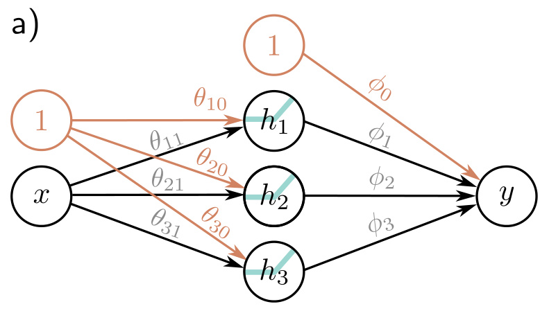
The intercepts, the ReLU functions and the parameter names are usually omitted from such
diagrams. The simpler depiction represents the same network; a reader who wants the
equation must supply the omitted parts from the convention rather than from the picture.
::: {.callout-note collapse="true" title="Outcomes and concepts"}
**Learning outcomes**
- {{< badge outcome "construct-shallow-network" >}} Construct a shallow ReLU network and trace how it produces a piecewise linear function.
**Concepts**
- {{< badge concept "shallow-neural-network" >}} one hidden layer of units, each a clipped linear function of the input, combined by a linear output function
- {{< badge concept "relu-activation-function" >}} $a[z] = \max(0, z)$ returns its input when positive and zero otherwise, which is what makes the network's output piecewise rather than linear
- {{< badge concept "linear-regions-and-joints" >}} each hidden unit contributes one joint at $x = -\theta_{d0}/\theta_{d1}$, so $D$ units give at most $D+1$ linear regions
- {{< badge concept "pre-activations-and-activations" >}} a unit whose pre-activation is negative is clipped and contributes nothing to the slope of that region
:::
## The universal approximation theorem
Generalising the example from three hidden units to $D$, the $d$-th hidden unit is
$$h_d = a[\theta_{d0} + \theta_{d1}x],$$
and these are combined linearly to create the output:
$$y = \phi_0 + \sum_{d=1}^{D}\phi_d h_d.$$
The number of hidden units in a shallow network is a measure of the **network capacity**.
With ReLU activations, the output of a network with $D$ hidden units has at most $D$
joints, and so is a piecewise linear function with at most $D + 1$ linear regions. Adding
hidden units allows the model to approximate more complex functions.
The informal argument for arbitrary accuracy follows from that count. Every additional
hidden unit adds one linear region to the function. As the regions become more numerous
they each represent a smaller section of the target function, and a smaller section of a
continuous function is increasingly well approximated by a line.
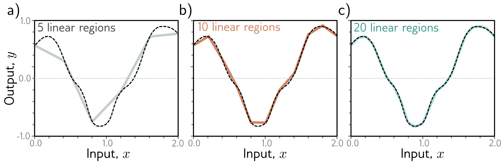
The **universal approximation theorem** makes the claim precise: for any continuous
function, there exists a shallow network that can approximate this function to any
specified precision. The statement generalises beyond the scalar case — with enough
hidden units, a shallow network can describe any continuous function defined on a compact
subset of $\mathbb{R}^{D_i}$ to arbitrary precision.
Three things the theorem does not say are worth stating explicitly, because each is a
common misreading.
- It does not bound the number of hidden units required.
> The theorem asserts existence. For some target functions the number of hidden units needed is impracticably large, and that observation is the motivation for depth.
- It does not provide the parameters, nor any procedure for finding them.
> A network approximating the target function to the required precision exists in the family. Locating it is a search over the parameter space, and the theorem is silent about whether that search succeeds.
- It says nothing about behaviour away from the data.
> Approximating a function on a compact domain to arbitrary precision is not the same claim as generalizing from a finite training sample, which is a matter of test error rather than representational capacity.
::: {.column-margin}
The *width version* of the theorem states that there exists a network with one hidden
layer containing a finite number of hidden units that can approximate any specified
continuous function on a compact subset of $\mathbb{R}^n$ to arbitrary accuracy. It was
proved by Cybenko (1989) for a class of sigmoid activations, and later shown by Hornik
(1991) to hold for a larger class of nonlinear activation functions.
:::
::: {.callout-note collapse="true" title="Outcomes and concepts"}
**Learning outcomes**
- {{< badge outcome "apply-universal-approximation" >}} State the universal approximation theorem and say what it does and does not promise.
**Concepts**
- {{< badge concept "universal-approximation-theorem" >}} for any continuous function on a compact domain there exists a shallow network approximating it to any specified precision, which is an existence claim and nothing more
- {{< badge concept "network-capacity" >}} the number of hidden units is the network's capacity, and it is what the approximation argument increases
- {{< badge concept "linear-regions-and-joints" >}} $D$ hidden units give at most $D$ joints and $D+1$ regions, so each added unit refines the piecewise linear approximation by one segment
:::
## Multivariate inputs and outputs
The universal approximation theorem holds for the general case, in which the network maps
multivariate inputs $\mathbf{x} = [x_1, x_2, \ldots, x_{D_i}]^T$ to multivariate
predictions $\mathbf{y} = [y_1, y_2, \ldots, y_{D_o}]^T$. Both extensions widen the weight
matrices and leave the mechanism untouched.
### Several outputs share the joints
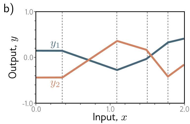
Multiple outputs are obtained by using a different linear function of the hidden units for
each output. A network with a scalar input $x$, four hidden units $h_1, \ldots, h_4$ and a
two-dimensional output $\mathbf{y} = [y_1, y_2]^T$ has hidden units $h_d = a[\theta_{d0} +
\theta_{d1}x]$ for $d = 1, \ldots, 4$, and outputs
$$y_1 = \phi_{10} + \phi_{11}h_1 + \phi_{12}h_2 + \phi_{13}h_3 + \phi_{14}h_4, \qquad y_2 = \phi_{20} + \phi_{21}h_1 + \phi_{22}h_2 + \phi_{23}h_3 + \phi_{24}h_4.$$
The joints of a piecewise linear output depend on where the initial linear functions
$\theta_{\bullet 0} + \theta_{\bullet 1}x$ are clipped at the hidden units. Since $y_1$
and $y_2$ are different linear functions of the *same* four hidden units, the four joints
of each must be in the same places. The slopes of the linear regions and the overall
vertical offset can differ.
### Several inputs make the joints into hyperplanes
Multivariate inputs are accommodated by extending the linear relation between the input
and each hidden unit. A network with two inputs $\mathbf{x} = [x_1, x_2]^T$ and a scalar
output has hidden units with one slope parameter per input:
$$h_1 = a[\theta_{10} + \theta_{11}x_1 + \theta_{12}x_2], \quad h_2 = a[\theta_{20} + \theta_{21}x_1 + \theta_{22}x_2], \quad h_3 = a[\theta_{30} + \theta_{31}x_1 + \theta_{32}x_2],$$
combined as $y = \phi_0 + \phi_1 h_1 + \phi_2 h_2 + \phi_3 h_3$.
Each hidden unit now receives a linear combination of the two inputs, which forms an
oriented plane in the three-dimensional input/output space. The activation function clips
the negative values of these planes to zero, and the clipped planes are recombined by the
output function into a continuous piecewise linear surface consisting of convex polygonal
regions. Each region corresponds to a different activation pattern; in the central
triangular region of the figure below, the first and third hidden units are active and the
second is inactive.
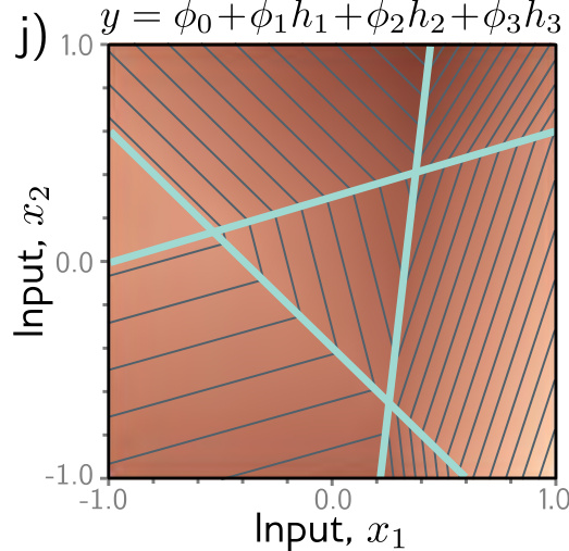
With more than two inputs the picture cannot be drawn, but the interpretation is
unchanged: the output is a continuous piecewise linear function of the input whose linear
regions are convex polytopes in the multi-dimensional input space. Each hidden unit
defines a hyperplane separating the part of space where that unit is active from the part
where it is not.
The number of regions grows quickly with input dimension. If a model had as many hidden
units as input dimensions $D_i$, each hyperplane could be aligned with one of the
coordinate axes; for two input dimensions this divides space into four quadrants, for
three dimensions into eight octants, and for $D_i$ dimensions into $2^{D_i}$ orthants.
Shallow networks usually have more hidden units than input dimensions, and so typically
create more than $2^{D_i}$ linear regions.
::: {.column-margin}
The exact bound is combinatorial. For $D_i \ge 2$-dimensional inputs and $D$ hidden units,
the number of regions created by $D$ hyperplanes in $D_i$-dimensional space was shown by
Zaslavsky (1975) to be at most $\sum_{j=0}^{D_i}\binom{D}{j}$. As a rule of thumb, a
shallow network creates between $2^{D_i}$ and $2^{D}$ linear regions.
:::
### The general case, and its vocabulary
The general shallow network $\mathbf{y} = \mathbf{f}[\mathbf{x}, \boldsymbol{\phi}]$ maps
$\mathbf{x} \in \mathbb{R}^{D_i}$ to $\mathbf{y} \in \mathbb{R}^{D_o}$ using
$\mathbf{h} \in \mathbb{R}^{D}$ hidden units. Each hidden unit is
$$h_d = a\Big[\theta_{d0} + \sum_{i=1}^{D_i}\theta_{di}x_i\Big],$$
and these are combined linearly to create the output:
$$y_j = \phi_{j0} + \sum_{d=1}^{D}\phi_{jd}h_d.$$
Counting the parameters is a matter of counting the coefficients in these two equations.
Each of the $D$ hidden units carries $D_i$ slopes and one offset; each of the $D_o$
outputs carries $D$ slopes and one offset. The total is therefore
$$(D_i + 1)D + (D + 1)D_o.$$
A network with three inputs, three hidden units and two outputs has fifteen slopes and
five offsets, twenty parameters in all.
The terminology is fixed here and reused for every architecture that follows. The left of
the diagram is the **input layer**, the centre is the **hidden layer**, and the right is
the **output layer**; the network below has one hidden layer containing four hidden units.
The hidden units are sometimes termed **neurons**. The values entering the hidden layer,
before the activation function is applied, are the **pre-activations**; the values at the
hidden layer, after it is applied, are the **activations**. The slope parameters are the
network **weights** and the offset parameters are the **biases**.
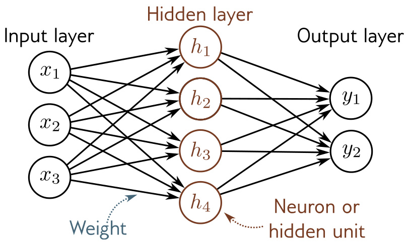
Any network with at least one hidden layer is also termed a **multi-layer perceptron**, or
**MLP**. A network with one hidden layer is a **shallow neural network**; one with
multiple hidden layers is a **deep neural network**. A network whose connections form an
acyclic graph is **feed-forward**, and one in which every element of a layer connects to
every element of the next is **fully connected**.
::: {.callout-tip title="Why the activation function must be nonlinear" collapse="true"}
The activation function permits the model to describe nonlinear relations between input
and output, and so it must be nonlinear itself. With no activation function, or with a
linear one, the overall mapping from input to output would be restricted to be linear:
a linear function of a linear function is again linear, and the hidden layer would buy
nothing.
The ReLU has the disadvantage that its derivative is zero for negative inputs. If every
training example produces a negative input to a given ReLU, the parameters feeding that
unit cannot be improved during training, because the gradient with respect to the incoming
weights is locally flat. This is the **dying ReLU** problem. Variants proposed to resolve
it include the leaky ReLU, which has a linear output of small slope for negative values;
the parametric ReLU, which treats that slope as an unknown parameter; and smooth
alternatives such as SoftPlus, GELU, SELU and Swish. No definitive answer exists as to
which is empirically superior, and these notes stay with the plain ReLU because the
functions it creates are easy to characterise in terms of their linear regions.
:::
::: {.highlights}
<h1>Key ideas</h1>
- A shallow network computes several linear functions of the input, passes each result through an activation function, and takes a linear combination of these activations to form the outputs.
- Multiple outputs share the hidden units and therefore share their joint positions; only slopes and offsets differ.
- With multivariate inputs the joints become hyperplanes, and the linear regions become convex polytopes on which the function is linear.
- A network with $D_i$ inputs, $D$ hidden units and $D_o$ outputs has $(D_i + 1)D + (D + 1)D_o$ parameters.
:::
::: {.callout-note collapse="true" title="Outcomes and concepts"}
**Learning outcomes**
- {{< badge outcome "generalize-multivariate" >}} Extend a shallow network to multivariate inputs and outputs and count its parameters.
- {{< badge outcome "construct-shallow-network" >}} Construct a shallow ReLU network and trace how it produces a piecewise linear function.
**Concepts**
- {{< badge concept "shallow-neural-network" >}} the general form is $h_d = a[\theta_{d0} + \sum_i \theta_{di}x_i]$ followed by $y_j = \phi_{j0} + \sum_d \phi_{jd}h_d$, for any input and output dimension
- {{< badge concept "linear-regions-and-joints" >}} with several inputs each unit's joint is a hyperplane, and the intersections of those hyperplanes cut the input space into convex polytopes
- {{< badge concept "pre-activations-and-activations" >}} the values entering the activation function are the pre-activations and those leaving it are the activations
- {{< badge concept "universal-approximation-theorem" >}} the guarantee carries over unchanged to multivariate inputs and outputs on a compact domain
- {{< badge concept "dying-relu-problem" >}} a ReLU receiving only negative pre-activations has zero gradient with respect to its incoming weights, so those weights cannot be improved
:::
## Composing networks into depth
Feeding the output of one shallow network into the input of a second is the shortest route
to understanding depth. Take two shallow networks with three hidden units each. The first
takes input $x$ and returns output $y$:
$$h_1 = a[\theta_{10} + \theta_{11}x], \quad h_2 = a[\theta_{20} + \theta_{21}x], \quad h_3 = a[\theta_{30} + \theta_{31}x],$$
$$y = \phi_0 + \phi_1 h_1 + \phi_2 h_2 + \phi_3 h_3.$$
The second takes $y$ as input and returns $y'$, with its own parameters:
$$h'_1 = a[\theta'_{10} + \theta'_{11}y], \quad h'_2 = a[\theta'_{20} + \theta'_{21}y], \quad h'_3 = a[\theta'_{30} + \theta'_{31}y],$$
$$y' = \phi'_0 + \phi'_1 h'_1 + \phi'_2 h'_2 + \phi'_3 h'_3.$$
With ReLU activations this composed model also describes a family of piecewise linear
functions. The number of linear regions, however, is potentially greater than for a
shallow network with six hidden units.
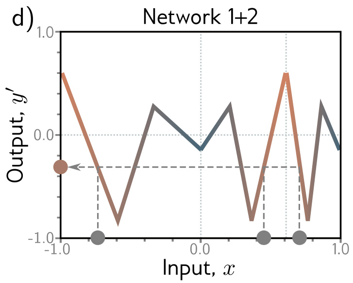
The reason is a counting argument. Choose the first network so that it produces three
alternating regions of positive and negative slope. Three different ranges of $x$ are then
mapped to the same output range $y \in [-1, 1]$, and the subsequent mapping from that range
of $y$ to $y'$ is applied three times. The function defined by the second network is
duplicated three times, variously flipped and rescaled according to the slope of the
regions of the first, to create nine linear regions.
![Composing two three-unit networks. b) the first network maps $x \in [-1,1]$ to $y \in [-1,1]$ with three alternating regions; c) the second network's function on $y$; d) the composition, in which the second network's function is duplicated three times, variously flipped and rescaled.](chapter_4_deep_neural_networks/img-3.jpeg)
The same principle applies in higher dimensions. Composing the two-input, three-unit
network of the previous section — whose output has seven linear regions, one of them flat
— with a second network of two hidden units, whose function on $y$ has two linear regions,
divides each of the six non-flat regions in two, for a total of thirteen linear regions.
### Folding
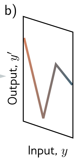
A second reading of the same composition is geometric. The first network **folds** the
input space $x$ back on top of itself, so that multiple inputs generate the same output.
The second network then applies a function, which is replicated at all the points that
were folded on top of one another.
### The composition is a two-layer network
The composition is not a new kind of object. The output of the first network, $y = \phi_0
+ \phi_1 h_1 + \phi_2 h_2 + \phi_3 h_3$, is a linear combination of the activations at the
hidden units, and the first operations of the second network — computing $\theta'_{10} +
\theta'_{11}y$ and its counterparts — are linear in that output. Applying one linear
function to another yields another linear function. Substituting the expression for $y$
into the second network's pre-activations gives
$$h'_1 = a[\theta'_{10} + \theta'_{11}\phi_0 + \theta'_{11}\phi_1 h_1 + \theta'_{11}\phi_2 h_2 + \theta'_{11}\phi_3 h_3],$$
with analogous expressions for $h'_2$ and $h'_3$, which can be rewritten as
$$h'_1 = a[\psi_{10} + \psi_{11}h_1 + \psi_{12}h_2 + \psi_{13}h_3],$$
where $\psi_{10} = \theta'_{10} + \theta'_{11}\phi_0$, $\psi_{11} = \theta'_{11}\phi_1$,
$\psi_{12} = \theta'_{11}\phi_2$, and so on. The result is a network with two hidden
layers.
::: {.callout-important title="The two-layer network is strictly larger than the composition"}
A network with two layers can represent the family of functions created by passing the
output of one single-layer network into another. It represents a *broader* family. In the
rewritten equations the nine slope parameters $\psi_{11}, \psi_{21}, \ldots, \psi_{33}$ can
take arbitrary values; in the composition they are constrained to be the outer product
$[\theta'_{11}, \theta'_{21}, \theta'_{31}]^T[\phi_1, \phi_2, \phi_3]$. Composition is the
special case; the deep network is the general one.
:::
::: {.callout-note collapse="true" title="Outcomes and concepts"}
**Learning outcomes**
- {{< badge outcome "compose-into-deep-networks" >}} Compose layers into a deep network and explain how folding multiplies linear regions.
:::
## Deep networks in matrix notation
The general two-hidden-layer network with three units per layer is written out in full as
a first layer
$$h_1 = a[\theta_{10} + \theta_{11}x], \qquad h_2 = a[\theta_{20} + \theta_{21}x], \qquad h_3 = a[\theta_{30} + \theta_{31}x],$$
a second layer
$$h'_1 = a[\psi_{10} + \psi_{11}h_1 + \psi_{12}h_2 + \psi_{13}h_3], \quad h'_2 = a[\psi_{20} + \psi_{21}h_1 + \psi_{22}h_2 + \psi_{23}h_3], \quad h'_3 = a[\psi_{30} + \psi_{31}h_1 + \psi_{32}h_2 + \psi_{33}h_3],$$
and an output
$$y' = \phi'_0 + \phi'_1 h'_1 + \phi'_2 h'_2 + \phi'_3 h'_3.$$
The construction proceeds in four steps. The three hidden units of the first layer are
computed as usual, by forming linear functions of the input and passing them through ReLU
activations. The pre-activations at the second layer are then three new linear functions of
those hidden units — at this point the object is a shallow network with three outputs, so
the three piecewise linear functions have their joints in the same places. A second ReLU
is applied to each, clipping them and adding new joints. The final output is a linear
combination of the second layer's hidden units.
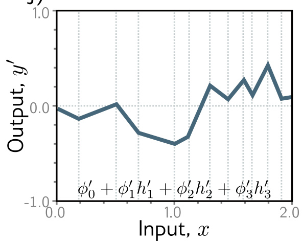
Each layer can therefore be read either as folding the input space or as creating new
functions which are clipped and recombined. The first view emphasises the dependencies
between regions in the output function; the second emphasises how clipping creates new
joints. Both are partial. What the network is, without metaphor, is an equation relating
input $x$ to output $y'$.
### The general formulation
The explicit notation becomes unmanageable beyond a few layers. Writing $\mathbf{h}_k$ for
the vector of hidden units at layer $k$, $\boldsymbol{\beta}_k$ for the biases that
contribute to layer $k+1$, and $\boldsymbol{\Omega}_k$ for the weights applied to the
$k$-th layer, a general deep network $\mathbf{y} = \mathbf{f}[\mathbf{x},
\boldsymbol{\phi}]$ with $K$ layers is
$$\mathbf{h}_1 = \mathbf{a}[\boldsymbol{\beta}_0 + \boldsymbol{\Omega}_0\mathbf{x}], \qquad \mathbf{h}_{k} = \mathbf{a}[\boldsymbol{\beta}_{k-1} + \boldsymbol{\Omega}_{k-1}\mathbf{h}_{k-1}], \qquad \mathbf{y} = \boldsymbol{\beta}_K + \boldsymbol{\Omega}_K\mathbf{h}_K,$$
where $\mathbf{a}[\bullet]$ applies the activation function separately to every element of
its vector input. The parameters $\boldsymbol{\phi}$ comprise all of these weight matrices
and bias vectors, $\boldsymbol{\phi} = \{\boldsymbol{\beta}_k, \boldsymbol{\Omega}_k\}_{k=0}^{K}$.
The dimensions are forced by the widths of the layers. If the $k$-th layer has $D_k$
hidden units, then the bias vector $\boldsymbol{\beta}_{k-1}$ is of size $D_k$, and the
last bias vector $\boldsymbol{\beta}_K$ has the size $D_o$ of the output. The first weight
matrix $\boldsymbol{\Omega}_0$ has size $D_1 \times D_i$; the last weight matrix
$\boldsymbol{\Omega}_K$ is $D_o \times D_K$; and the remaining matrices
$\boldsymbol{\Omega}_k$ are $D_{k+1} \times D_k$.
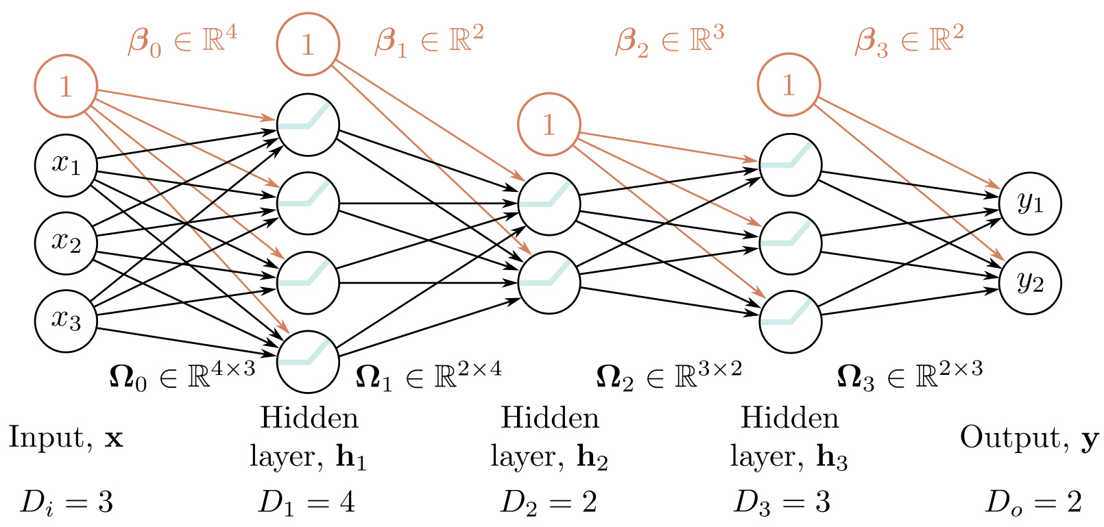
For that network the weight matrices contribute $4 \times 3 + 2 \times 4 + 3 \times 2 + 2
\times 3 = 32$ parameters and the bias vectors contribute $4 + 2 + 3 + 2 = 11$, for
$43$ in total. Hidden layers need not have equal widths, and in this example none of the
three does.
### Parameters and hyperparameters
Two kinds of quantity have now appeared, and conflating them is the standard error at this
point.
- The **parameters** $\boldsymbol{\phi} = \{\boldsymbol{\beta}_k, \boldsymbol{\Omega}_k\}$ are learned by minimizing a loss.
> They are the weights and biases, and they are what training searches over.
- The **hyperparameters** are the number of layers $K$ and the number of hidden units in each layer, $D_1, D_2, \ldots, D_K$.
> They are chosen before the model parameters are learned. The number of hidden units in each layer is termed the **width** of the network, the number of hidden layers its **depth**, and the total number of hidden units a measure of its **capacity**.
For fixed hyperparameters — two layers with three hidden units each, say — the model
describes a family of functions, and the parameters determine the particular member. Taking
the hyperparameters into account as well, a neural network represents a family of families
of functions relating input to output.
::: {.callout-note title="Representability is not the interesting question"}
A deep network with two hidden layers can represent the composition of two shallow
networks. If the second of those networks computes the identity function, the deep network
replicates a single shallow network. A deep network therefore inherits the shallow
network's universal approximation property, and can approximate any continuous function
arbitrarily closely given sufficient capacity. Both families being universal
approximators, the question that separates them is not what can be represented but at what
cost.
:::
::: {.callout-note collapse="true" title="Outcomes and concepts"}
**Learning outcomes**
- {{< badge outcome "write-matrix-form" >}} Write a $K$-layer network in matrix notation and name its hyperparameters.
- {{< badge outcome "compose-into-deep-networks" >}} Compose layers into a deep network and explain how folding multiplies linear regions.
**Concepts**
- {{< badge concept "matrix-formulation" >}} a $K$-layer network computes each layer as $\mathbf{h}_k = \mathbf{a}[\boldsymbol{\beta}_{k-1} + \boldsymbol{\Omega}_{k-1}\mathbf{h}_{k-1}]$, with matrix shapes fixed by the layer widths
- {{< badge concept "deep-neural-network" >}} more than one hidden layer, specified by arbitrary depth and per-layer widths, and reducible to a single equation from input to output
- {{< badge concept "network-hyperparameters" >}} depth $K$ and width $D_k$ are fixed before training and select the family of functions the parameters then range over
:::
## Shallow against deep
Both families can approximate any continuous function given enough capacity, so
approximation power alone does not decide between them. Four further comparisons do the
work, and the first two are theoretical while the last two are empirical.
### Linear regions per parameter
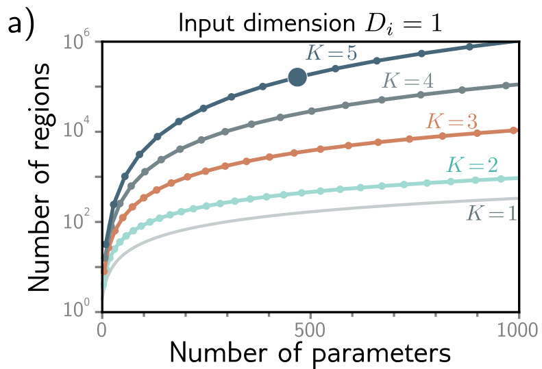
A shallow network with one input, one output and $D > 2$ hidden units can create up to
$D + 1$ linear regions and is defined by $3D + 1$ parameters. A deep network with one
input, one output and $K$ layers of $D > 2$ hidden units can create a function with up to
$(D+1)^K$ linear regions using $3D + 1 + (K-1)D(D+1)$ parameters.
The difference is the difference between adding and multiplying. A network with $K = 5$
layers of $D = 10$ hidden units has $471$ parameters and can produce $161{,}051$ regions.
A shallow network with the same parameter budget produces of the order of $150$. The effect
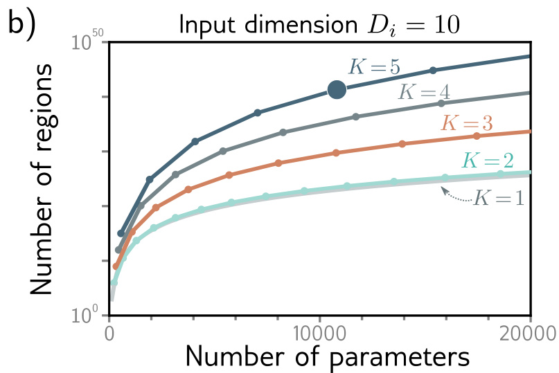
is magnified as the input dimension grows: with $D_i = 10$, a model with $K = 5$ layers of
$D = 50$ hidden units has $10{,}801$ parameters and can create more than $10^{40}$ linear
regions.
:::: {.columns}
::: {.column width="48%"}
:::
::: {.column width="48%"}
:::
::::
The count alone overstates the case, and the source is explicit about why. The flexibility
of the functions remains limited by the number of parameters. Deep networks create
extremely large numbers of linear regions, but those regions contain complex dependencies
and symmetries — visible in the folding picture, where the pattern drawn on the folded
sheet is stamped out identically on every fold. A greater number of regions is therefore
not clearly an advantage unless there are similar symmetries in the real-world functions
to be approximated, or there is reason to believe that the mapping from input to output
genuinely involves a composition of simpler functions.
### Depth efficiency
**Depth efficiency** is the property that some functions can be approximated much more
efficiently by deep networks than by shallow ones. Functions have been identified that
require a shallow network with exponentially more hidden units to achieve an approximation
equivalent to that of a deep network. As with the region count, it is not established that
the real-world functions one wants to approximate fall into this category.
### Large structured inputs
Fully connected networks, in which every element of each layer contributes to every
element of the next, are not practical for large structured inputs such as images, where
the input might comprise around $10^6$ pixels. The number of parameters would be
prohibitive. There is a second objection, independent of cost: different parts of an image
should be processed similarly, and there is no point in independently learning to recognise
the same object at every possible position in the image.
The alternative is to process local image regions in parallel and then gradually integrate
information from increasingly large regions. This local-to-global processing is difficult
to specify without using multiple layers.
### Training and generalization
Two empirical observations complete the comparison, and both are reported as observations
rather than as results.
- Moderately deep networks are usually easier to train than shallow ones.
> One conjecture is that over-parameterized deep models — those with more parameters than training examples — possess a large family of roughly equivalent solutions that are easy to find. As more hidden layers are added, training becomes more difficult again, and methods for mitigating that are the subject of later material.
- Deep networks appear to generalize to new data better than shallow ones.
> In practice the best results for most tasks have been achieved using networks with tens or hundreds of layers. Neither this phenomenon nor the preceding one is well understood.
::: {.highlights}
<h1>Key ideas</h1>
- Both shallow and deep networks can approximate any continuous function given enough capacity, so the comparison must be made on cost rather than on representability.
- Deep networks produce many more linear regions per parameter, but those regions carry dependencies and symmetries that a raw count ignores.
- Depth efficiency is a proven property of certain functions, not a demonstrated property of the functions encountered in applications.
- Large structured inputs such as images require local-to-global processing, which needs multiple layers.
- Deep networks are empirically easier to train up to a point and appear to generalize better; neither observation has a settled explanation.
:::
::: {.callout-note collapse="true" title="Outcomes and concepts"}
**Learning outcomes**
- {{< badge outcome "compare-depth-and-width" >}} Compare deep and shallow networks on expressivity per parameter and on practical trainability.
- {{< badge outcome "apply-universal-approximation" >}} State the universal approximation theorem and say what it does and does not promise.
- {{< badge outcome "evaluate-generalization" >}} Distinguish training error from test error and diagnose underfitting versus overfitting.
**Concepts**
- {{< badge concept "universal-approximation-theorem" >}} a deep network can replicate a shallow one by computing the identity in its second layer, and so inherits the approximation guarantee
- {{< badge concept "linear-regions" >}} a deep network of $K$ layers of $D$ units reaches $(D+1)^K$ regions on $3D + 1 + (K-1)D(D+1)$ parameters, against $D+1$ regions on $3D+1$ for a shallow one
- {{< badge concept "space-folding" >}} folding explains both why regions multiply with depth and why they are not independent of one another
- {{< badge concept "depth-efficiency" >}} certain functions require exponentially more hidden units in a shallow network than in a deep one for an equivalent approximation
- {{< badge concept "deep-neural-network" >}} depth is favoured for its regions per parameter, its suitability for local-to-global processing, and its observed trainability and generalization
:::
## What this unit establishes
- Supervised learning maps inputs to outputs using a parameterized function learned from example data.
> The template — model, loss, training — is fixed once and reused for every family that follows.
- Model training is the optimization of parameters to minimize a loss function such as the least-squares error.
> The loss is a surface over the parameter space, and training is a descent on that surface from a random start.
- A trained model is evaluated on unseen test data, balancing underfitting against overfitting.
> A low training loss is compatible with both a well-matched model and one that has fitted the sample's noise, so it cannot settle the question by itself.
- 1D linear regression illustrates the whole workflow in a form that can be drawn.
> Two parameters make the loss surface a visible object rather than an abstraction, which is what makes the example worth the space.
- Shallow ReLU networks construct continuous piecewise linear functions from input space to output space.
> Each hidden unit contributes one joint, and the activation pattern of the units determines the slope of each region.
- The universal approximation theorem establishes that a shallow network of sufficient capacity approximates any continuous function to arbitrary precision.
> It is an existence result. It bounds neither the width required nor the difficulty of the search for the parameters.
- Shallow networks extend to multivariate inputs and outputs by widening the weight matrices.
> Outputs sharing hidden units share their joints; inputs of dimension $D_i$ turn joints into hyperplanes and regions into convex polytopes.
- Nonlinear activations are what make depth expressive, and the choice among them affects gradient behaviour during training.
> Without a nonlinearity the composition of layers collapses to a single linear map, and the ReLU's zero gradient on negative inputs is the price of its simplicity.
- Deep networks generate exponentially more linear regions per parameter than shallow networks, through composition and the folding of input space.
> The regions are not independent, so the count is an upper bound on flexibility rather than a measure of it.
- Deep network computation generalizes to alternating matrix multiplications, bias additions and element-wise nonlinearities.
> Depth and width are hyperparameters fixed before training; the weights and biases are the parameters training searches over.
- Depth carries a theoretical advantage in depth efficiency and practical advantages in training, generalization and the handling of structured data.
> The theoretical claims are proved for particular functions; the practical ones are empirical regularities without settled explanations.
Two things in this unit were asserted rather than derived. The least-squares loss was
introduced by stipulation, and the phrase *descend the loss surface* was left without an
algorithm behind it. *Training Models* supplies both. Loss functions are derived there
from maximum likelihood, so that least-squares and cross-entropy follow from a single
principle rather than from separate conventions; and the optimizers that minimize those
losses — stochastic gradient descent, momentum, Adam — are treated together with
backpropagation, the algorithm that computes the gradients the networks of this unit
require.
## References
- Understanding Deep Learning, _Simon Prince_, 2026 — [Link](https://udlbook.github.io/udlbook/) — Pages 31-38, 39-54, 55-69
::: {.hg-nav}
[← Preliminaries to Machine Learning](index.qmd){.hg-prev}
[Training Models →](../training_models/index.qmd){.hg-next}
:::