Preliminaries to Machine Learning

Basics to Machine Learning · v1.1.43

2026-09-08 16:27:15

Where we are

The first unit of Basics to Machine Learning

Three prerequisites are used, and no others.

• The equation of a straight line, in terms of its intercept and slope.
• Matrix–vector multiplication, and the dimensions that make a product defined.
• The partial derivative, used only to give meaning to the gradient of a surface.

Nothing beyond these three is assumed anywhere in the unit. If a student is shaky on matrix shapes, the matrix-notation section later on is where it will bite.

One template organises the whole unit

• A model — a family of functions \(\mathbf{y} = \mathbf{f}[\mathbf{x}, \boldsymbol{\phi}]\), whose particular member is fixed by the parameters \(\boldsymbol{\phi}\).
• A loss — a scalar \(L[\boldsymbol{\phi}]\) measuring how badly a given choice of parameters predicts a training set.
• A training procedure — a search for the parameters at which the loss is small.

The three families treated below — the straight line, the shallow network, the deep network — differ in the first item and in nothing else.

The functional form is chosen by the designer; the parameters are not. Lower loss is better, and the loss is the only quantity training consults. Say the template once here and then point back at it in every section.

The supervised learning framework

A model is a mapping from inputs to outputs

A supervised learning model defines a mapping from one or more inputs to one or more outputs.

\[\mathbf{y} = \mathbf{f}[\mathbf{x}].\]

The worked case is the valuation of a second-hand car: the input is the car’s age and mileage, the output is its estimated value in dollars.

Input and output are vectors of predetermined, fixed size whose elements always appear in the same order — age first, then mileage, in every example. Data of this form is termed structured or tabular data.

The parameters belong in the notation

Computing \(\mathbf{y}\) from \(\mathbf{x}\) is termed inference.

The model is an equation of fixed form containing parameters \(\boldsymbol{\phi}\), so the honest form carries them explicitly:

\[\mathbf{y} = \mathbf{f}[\mathbf{x}, \boldsymbol{\phi}].\]

The equation names a family of relations; the parameters name one member of that family.

Training is a minimization

Learning or training means finding parameters that produce sensible predictions, using a training dataset of \(I\) pairs \(\{\mathbf{x}_i, \mathbf{y}_i\}\).

The loss \(L\) summarises how poorly the model with parameters \(\boldsymbol{\phi}\) predicts the training outputs, and training minimizes it:

\[\hat{\boldsymbol{\phi}} = \operatorname*{argmin}_{\boldsymbol{\phi}}\Big[L[\boldsymbol{\phi}]\Big].\]

Strictly, a loss function is the term for a single data point, a cost function the overall quantity minimized, and an objective function any function to be maximized or minimized. The first two are used interchangeably in most of the literature.

Two features easily missed

• The loss depends on the training data as well as on the parameters.
• A small loss after minimization establishes only that the model predicts the training outputs accurately.

Written in full the loss is \(L[\{\mathbf{x}_i, \mathbf{y}_i\}, \boldsymbol{\phi}]\). The data are suppressed from the notation because they are held fixed while the parameters vary, not because they are absent.

Performance is afterwards assessed on separate test data, to determine how well the model generalizes to examples it did not observe during training. Only if that performance is adequate is the model ready for deployment.

Inference is cheap; training is a search

Inference is a single evaluation of the function with the parameters held fixed.

Training searches the space of parameters for the value minimizing the loss.

That asymmetry holds for every model treated in this unit.

Discriminative and generative formulations

Discriminative

\[\mathbf{y} = \mathbf{f}[\mathbf{x}, \boldsymbol{\phi}]\]

Predicts the output directly from the measurement.

Generative

\[\mathbf{x} = \mathbf{g}[\mathbf{y}, \boldsymbol{\phi}]\]

Computes the measurement from the output; inference needs \(\mathbf{y} = \mathbf{g}^{-1}[\mathbf{x}, \boldsymbol{\phi}]\).

Prior knowledge — of 3D geometry or of optics, say — can be built into a generative model, but inverting it may be difficult. Discriminative models dominate modern practice: the advantage of built-in prior knowledge is usually outweighed by fitting very flexible discriminative models to large quantities of training data.

Linear regression and its loss surface

The straight-line family \(^1/_2\)

A 1D linear regression model relates a scalar input to a scalar output as a straight line:

\[y = \mathrm{f}[x, \boldsymbol{\phi}] = \phi_0 + \phi_1 x.\]

• Two parameters, \(\boldsymbol{\phi} = [\phi_0, \phi_1]\)
• \(\phi_0\) is the y-intercept, \(\phi_1\) the slope
• The equation defines all lines; the parameters select one

The straight-line family \(^2/_2\)

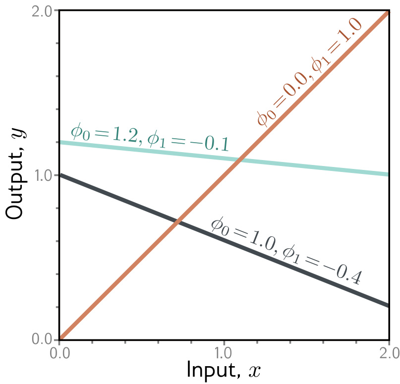
Three members of the family:

• \((\phi_0,\phi_1) = (1.2, -0.1)\)
• \((\phi_0,\phi_1) = (0.0, 1.0)\)
• \((\phi_0,\phi_1) = (1.0, -0.4)\)

One equation, one family of lines; the intercept and the slope pick out the member.

What the data offers, and what is wanted

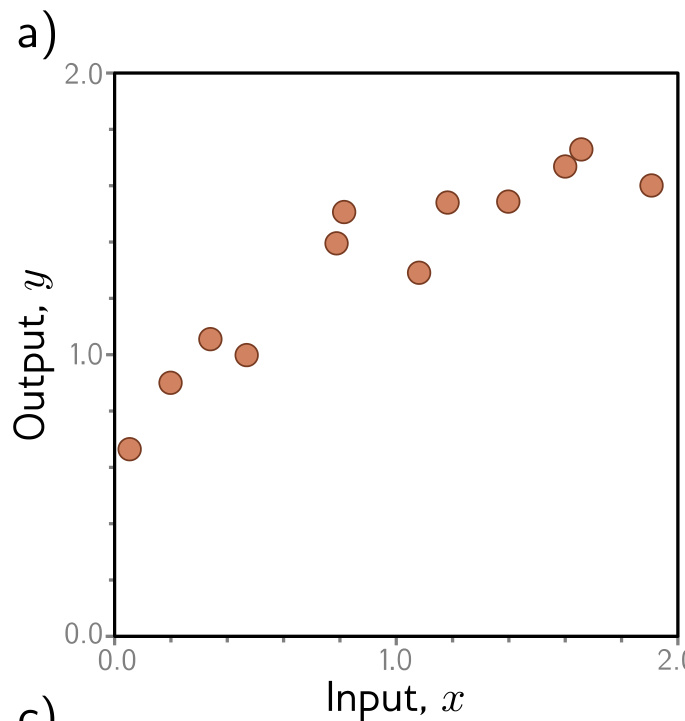
The data is \(I\) pairs \(\{x_i, y_i\}\), and nothing more.

• The model is discriminative: it predicts \(y\) from \(x\).
• Many lines fit the cloud somehow.
• A criterion must pick one.

This is the bridge from the family of lines to the loss. The family is infinite and the data is fixed, so the question is not what lines exist but which line the data favours. The alternative would be a generative account, modelling \(x\) as a function of \(y\) — that is a different model, and inference then requires inverting it.

The least-squares loss

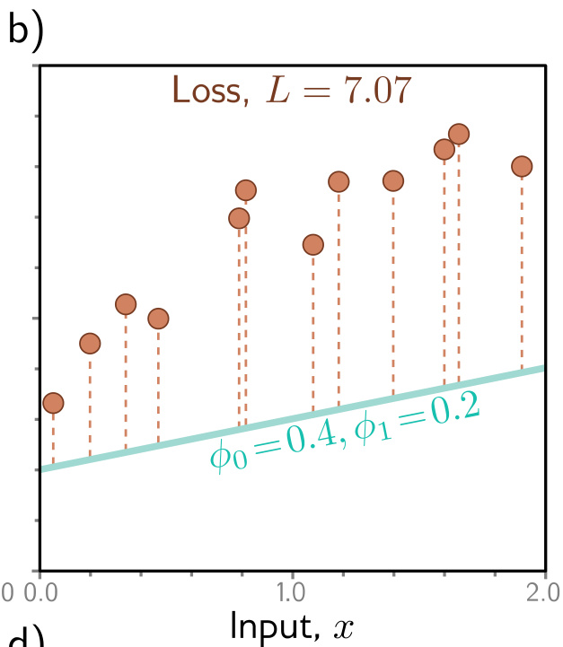
The mismatch at example \(i\) is the deviation between the height of the line at \(x_i\) and the observed output \(y_i\). The total, termed the training error, is

\[L[\boldsymbol{\phi}] \;=\; \sum_{i=1}^{I}\big(\mathrm{f}[x_i, \boldsymbol{\phi}] - y_i\big)^2 \;=\; \sum_{i=1}^{I}\big(\phi_0 + \phi_1 x_i - y_i\big)^2.\]

Because the best parameters minimize this expression, it is a least-squares loss.

The squaring makes the direction of the deviation immaterial: a point lying above the line is penalised exactly as much as a point the same distance below it. A probabilistic justification for this particular choice exists, and is the subject of the next unit.

Poor parameters and good ones

A poor fit, \(\phi_0 = 0.4, \phi_1 = 0.2\), giving \(L = 7.07\). The orange dashed segments are the deviations being squared.

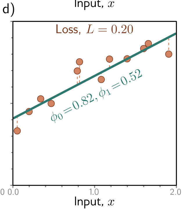
The optimal fit, \(\phi_0 = 0.82, \phi_1 = 0.52\), giving \(L = 0.20\).

\(L = 7.07\) against \(L = 0.20\).

A third line, \(\phi_0 = 1.60, \phi_1 = -0.8\), gives \(L = 10.28\). The value \(L = 0.20\) is the smallest loss attainable by any line on this data.

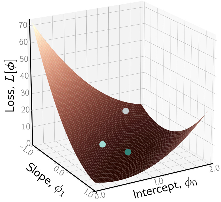
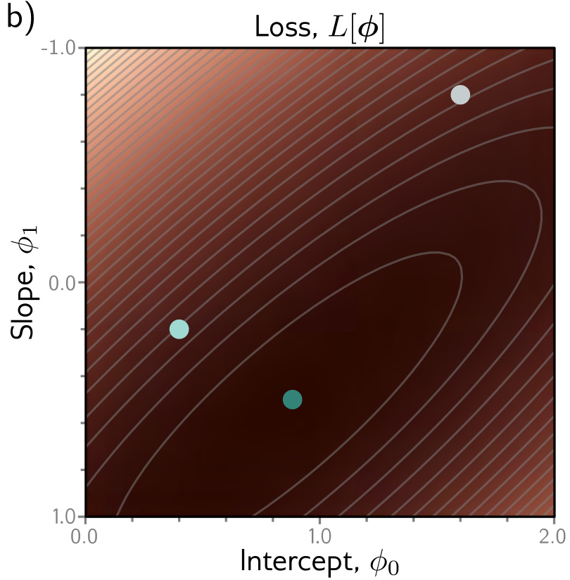
The loss is a surface over parameter space

\(L[\boldsymbol{\phi}]\) as a surface over intercept and slope.

The same surface from above. Brighter regions carry larger losses; the gray ellipses are isocontours.

Two parameters, so the whole surface can be drawn.

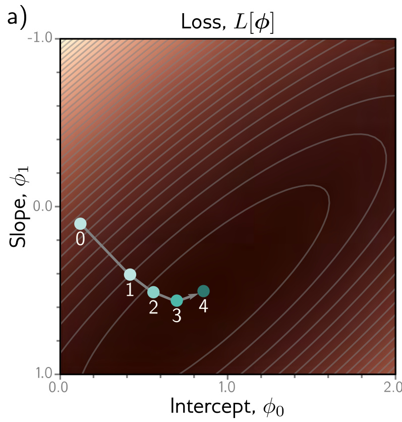
Training walks downhill on that surface

Positions 0 to 4, walking downhill.

• Start at random parameters
• Measure the gradient
• Step downhill
• Repeat until flat

Finding the parameters that minimize the loss is termed model fitting, training, or learning. All three names are in use for the same thing. The lines fit the data more closely as the loss decreases.

The iterative method is not needed here — and that is the point

This model

\(\partial L/\partial\phi_0\) and \(\partial L/\partial\phi_1\) can be set to zero and solved for the optimum in closed form.

Every model after it

No closed-form solution, and far too many parameters to evaluate the loss for every combination.

Descent is introduced for the second column, not the first.

Testing and generalization

The training loss is not the quantity of interest

Training loss

What the minimization returned. Measures performance on the training data alone.

Test loss

The same loss on a separate set of test data. Stands in for performance in the real world.

How well accuracy generalizes depends partly on the training data, partly on the model.

Two failure modes, and they are opposites

Underfitting

The model family is too restrictive to capture the true relationship.

Overfitting

A very expressive model describes atypical peculiarities of the training sample.

This is why model capacity — for a network, the number of hidden units — is a design decision rather than a quantity to be maximised.

A straight line fitted to data that curves is the standard case of underfitting: no choice of intercept and slope reduces the training loss much, and the deficiency lies in the family, not in the search.

Under overfitting the training loss can be driven very low precisely because the model has enough capacity to accommodate the noise in the particular sample. The training loss is then no longer evidence of anything.

What linear regression has established

• A model is \(\mathbf{y} = \mathbf{f}[\mathbf{x}, \boldsymbol{\phi}]\)
• A loss \(L[\boldsymbol{\phi}]\) scores the parameters against the data
• Training minimizes it; test data judges the result

The drawback: a straight line, and nothing else.

Shallow networks, next, are only slightly more complex than linear regression but describe a much larger family of relations. Deep networks are just as expressive as shallow ones, and describe complex functions with fewer parameters.

Shallow networks and piecewise linear functions

An example network with ten parameters

A shallow neural network has one hidden layer:

\[\begin{aligned} y = \mathrm{f}[x, \boldsymbol{\phi}] = \;& \phi_0 + \phi_1 a[\theta_{10} + \theta_{11}x] \\ &+ \phi_2 a[\theta_{20} + \theta_{21}x] + \phi_3 a[\theta_{30} + \theta_{31}x]. \end{aligned}\]

• Three linear functions of the input
• Each through an activation function \(a[\bullet]\)
• Weighted, summed, offset by \(\phi_0\)

The rectified linear unit

\[a[z] = \mathrm{ReLU}[z] = \begin{cases} 0 & z < 0 \\ z & z \ge 0. \end{cases}\]

It returns the input when the input is positive, and zero otherwise — it clips negative values to zero.

The ReLU is the only activation used in this unit. Its virtue here is that the functions it creates are easy to characterise in terms of their linear regions.

Hidden units and joints

Hidden units

\[\begin{aligned} h_1 &= a[\theta_{10} + \theta_{11}x] \\ h_2 &= a[\theta_{20} + \theta_{21}x] \\ h_3 &= a[\theta_{30} + \theta_{31}x] \end{aligned}\]

\(y = \phi_0 + \phi_1 h_1 + \phi_2 h_2 + \phi_3 h_3\)

Joints

Unit \(d\) switches where its linear function crosses zero:

\[x = -\frac{\theta_{d0}}{\theta_{d1}}\]

One joint per unit, so up to four linear regions.

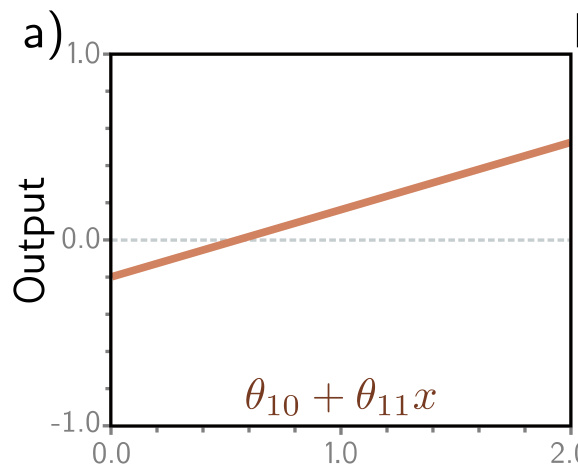
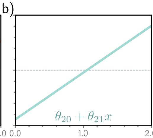
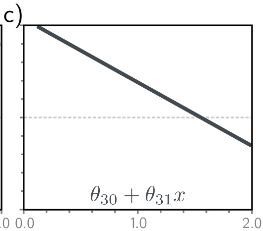
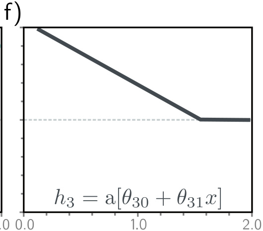
Stage 1: three linear functions

Each unit computes its own \(\theta_{d0} + \theta_{d1}x\) — its own intercept and slope.

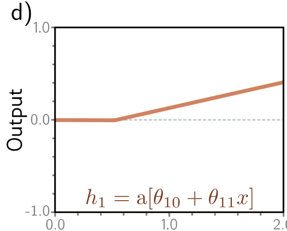
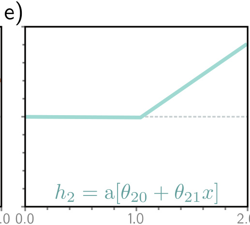
Stage 2: the ReLU clips each one

Negatives become zero. Each unit gains a joint where its line crossed zero.

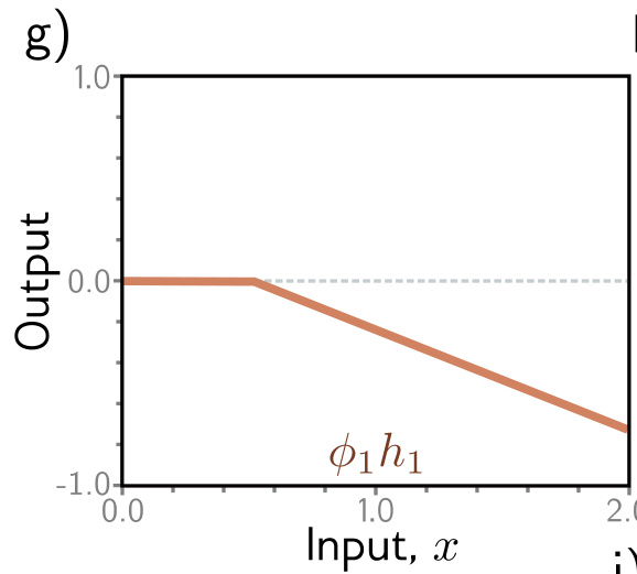
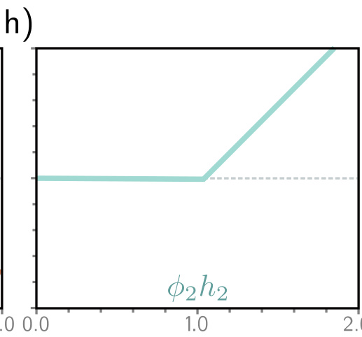
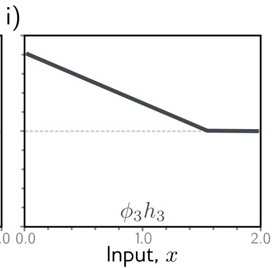
Stage 3: weight each activation

The output weights \(\phi_1, \phi_2, \phi_3\) scale and may flip each contribution.

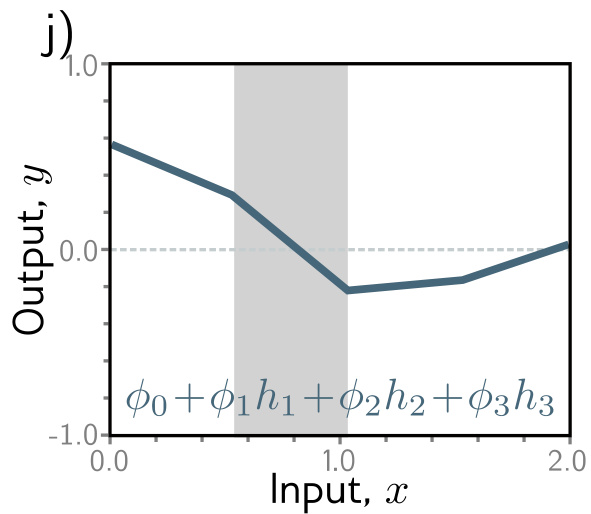
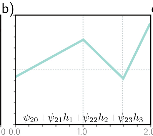
Stage 4: sum, and add the offset

• Three joints, four linear regions
• The shaded region: \(h_2\) inactive, \(h_1\) and \(h_3\) active
• \(\phi_0\) sets the overall height

Activation patterns set the slopes

Each linear region corresponds to a different activation pattern. A clipped unit is inactive; an unclipped unit is active.

The slope of a region comes from the slopes \(\theta_{\bullet 1}\) of the units active there, together with the output weights \(\phi_{\bullet}\) applied to them — in the shaded region, \(\theta_{11}\phi_1 + \theta_{31}\phi_3\).

Three units give four regions, but only three of the four slopes are independent.

The fourth slope is either zero — if every hidden unit is inactive in that region — or a sum of the slopes of the other regions. This is a standard misreading: four regions do not mean four degrees of freedom.

Reading the diagram

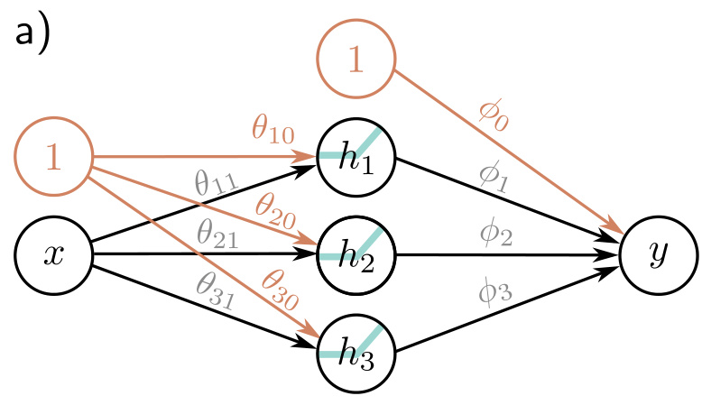
Intercepts in orange, slopes in black.

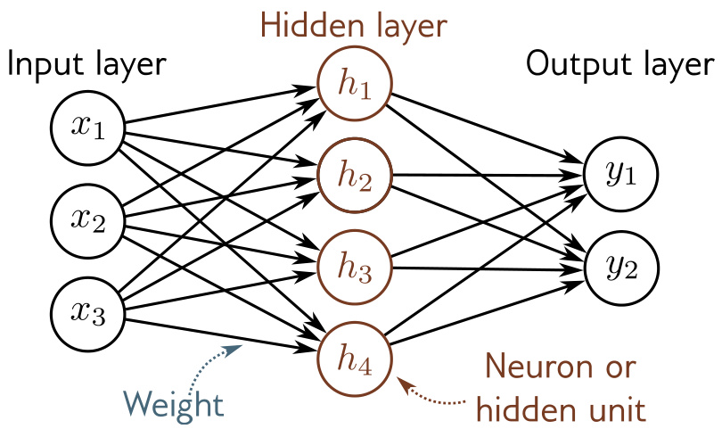
• Input left, hidden units centre, output right
• Each connection is one parameter
• Offsets enter as extra nodes holding one

Intercepts, ReLUs and parameter names are usually omitted — supplied by convention, not by the picture.

The universal approximation theorem

Generalising to \(D\) hidden units

\[h_d = a[\theta_{d0} + \theta_{d1}x], \qquad y = \phi_0 + \sum_{d=1}^{D}\phi_d h_d.\]

• \(D\) hidden units is the network capacity
• With ReLU, \(D\) units give at most \(D\) joints
• So at most \(D + 1\) linear regions

The informal argument

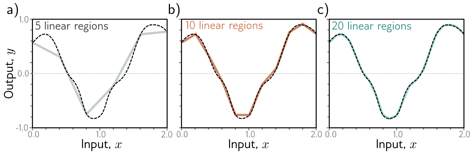
A 1D function (dashed) approximated by a piecewise linear model with 5, 10 and 20 linear regions.

• One more unit, one more region
• More regions, smaller sections each
• A small section of a curve is nearly a line

The claim, made precise

• For any continuous function
• On a compact subset of \(\mathbb{R}^{D_i}\)
• There exists a shallow network
• Approximating it to any specified precision

The width version of the theorem was proved by Cybenko (1989) for a class of sigmoid activations, and later shown by Hornik (1991) to hold for a larger class of nonlinear activation functions.

Three things the theorem does not say

• It does not bound the number of hidden units required.
• It does not provide the parameters, nor any procedure for finding them.
• It says nothing about behaviour away from the data.

The theorem asserts existence. For some target functions the number of hidden units needed is impracticably large, and that observation is the motivation for depth.

A network approximating the target to the required precision exists in the family; locating it is a search over the parameter space, and the theorem is silent about whether that search succeeds.

Approximating a function on a compact domain to arbitrary precision is not the same claim as generalizing from a finite training sample — that is a matter of test error rather than representational capacity.

Multivariate inputs and outputs

Both extensions widen the matrices

The theorem holds for the general case, mapping \(\mathbf{x} = [x_1, \ldots, x_{D_i}]^T\) to \(\mathbf{y} = [y_1, \ldots, y_{D_o}]^T\).

Widening the weight matrices leaves the mechanism untouched.

The two extensions, drawn

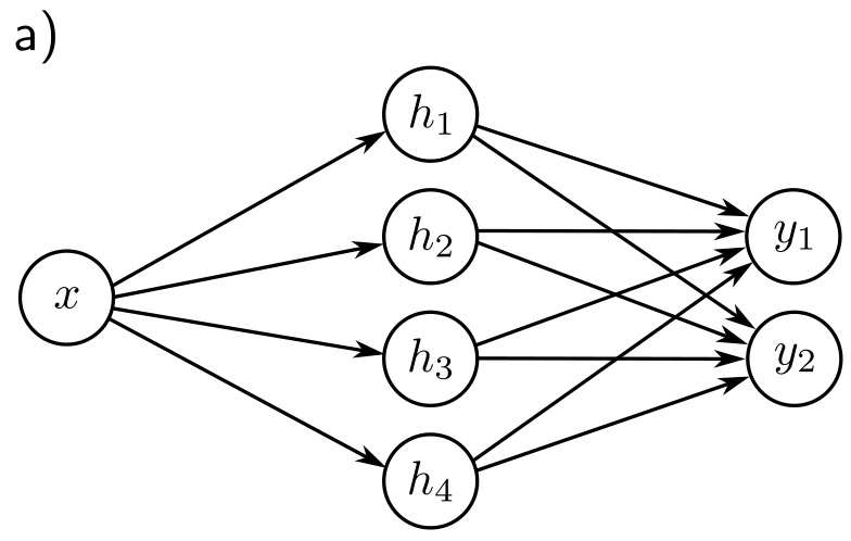
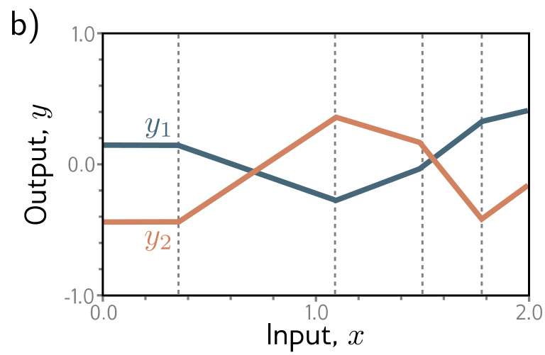
One input, four units, two outputs

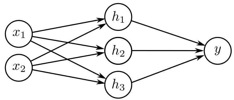
Two inputs, three units, one output

Outputs fan out on the right; inputs fan in on the left. The hidden layer is unchanged.

Several outputs share the joints

\[y_1 = \phi_{10} + \sum_{d=1}^{4}\phi_{1d}h_d, \qquad y_2 = \phi_{20} + \sum_{d=1}^{4}\phi_{2d}h_d.\]

• Each output reads the same hidden units
• So the joints (dotted) coincide
• Slopes and heights differ

The joints depend on where the initial linear functions are clipped at the hidden units. Since both outputs read the same four units, their four joints must be in the same places. Only the slopes of the regions and the overall vertical offset can differ.

Several inputs make the joints into hyperplanes

One slope parameter per input:

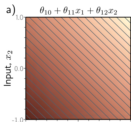
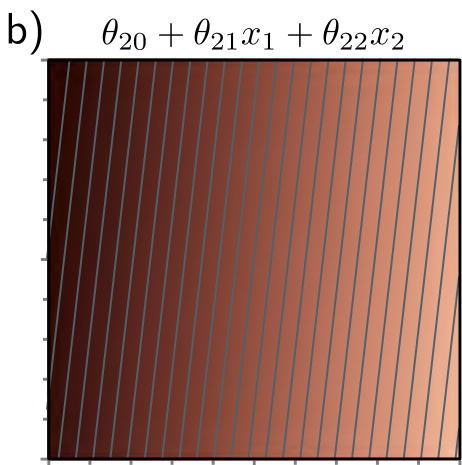
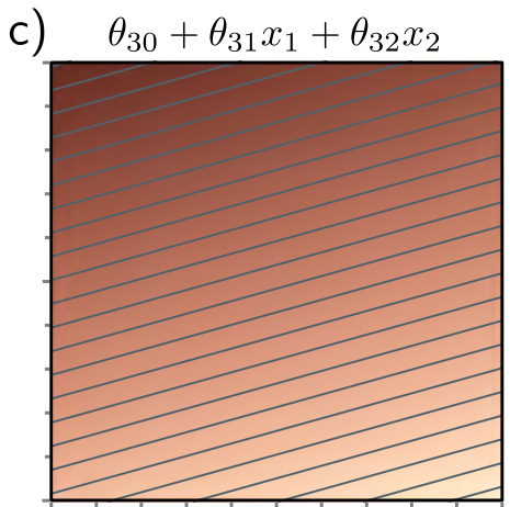
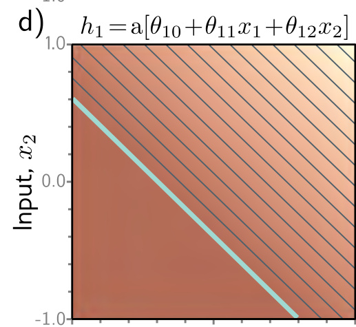
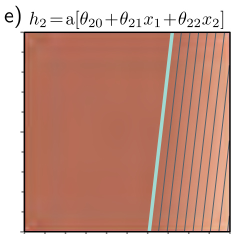
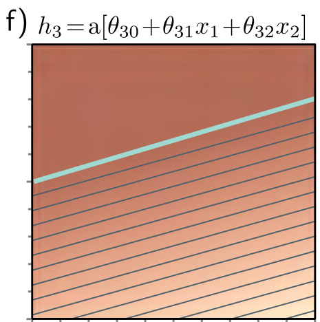
\[\begin{aligned} h_1 &= a[\theta_{10} + \theta_{11}x_1 + \theta_{12}x_2] \\ h_2 &= a[\theta_{20} + \theta_{21}x_1 + \theta_{22}x_2] \\ h_3 &= a[\theta_{30} + \theta_{31}x_1 + \theta_{32}x_2] \end{aligned}\]

• Each unit is an oriented plane
• The ReLU clips its negative half
• Summing gives a surface of convex polygonal regions

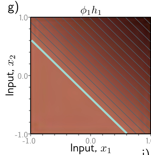
Stage 1: three oriented planes

Brightness is the unit’s output. Each is a plane tilted its own way.

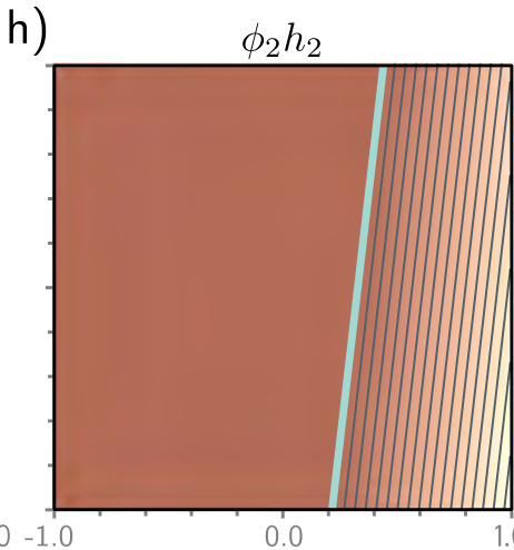
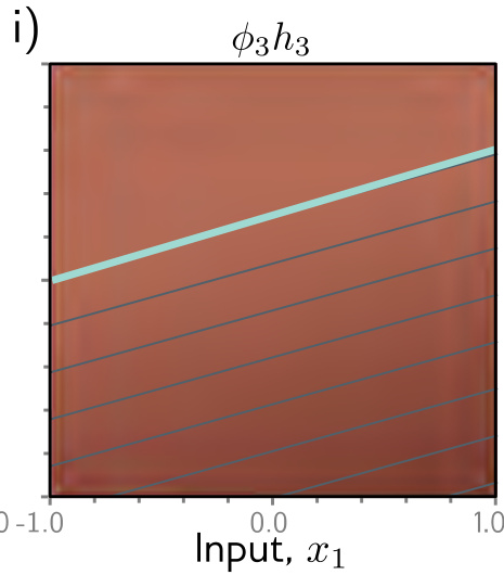
Stage 2: the ReLU cuts each plane

The cyan line is the joint — a hyperplane. One side is flat zero.

Stage 3: weight each clipped plane

Each contribution is scaled by \(\phi_1, \phi_2, \phi_3\).

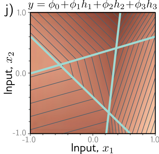
Stage 4: sum into a polygonal surface

• Three joints cut the plane into convex polygons
• The function is linear on each polygon
• Central triangle: \(h_1, h_3\) active, \(h_2\) inactive

The regions multiply with input dimension

Beyond two inputs

• The picture cannot be drawn
• Regions are convex polytopes
• Each unit is a hyperplane: active on one side

Counting them

• \(D = D_i\), axis-aligned: \(2^{D_i}\) orthants
• 4 quadrants in 2D, 8 octants in 3D

Shallow networks have more units than inputs, so typically more than \(2^{D_i}\) regions.

The exact bound is combinatorial: for \(D_i \ge 2\) and \(D\) hidden units, Zaslavsky (1975) showed the number of regions is at most \(\sum_{j=0}^{D_i}\binom{D}{j}\). As a rule of thumb, a shallow network creates between \(2^{D_i}\) and \(2^{D}\) linear regions.

The general case

\[h_d = a\Big[\theta_{d0} + \sum_{i=1}^{D_i}\theta_{di}x_i\Big], \qquad y_j = \phi_{j0} + \sum_{d=1}^{D}\phi_{jd}h_d.\]

Each of the \(D\) hidden units carries \(D_i\) slopes and one offset; each of the \(D_o\) outputs carries \(D\) slopes and one offset:

\[(D_i + 1)D + (D + 1)D_o.\]

Three inputs, three hidden units, two outputs: fifteen slopes and five offsets, twenty parameters in all.

The vocabulary, fixed here for good

A shallow network annotated with its layers, hidden units and weights.

• input, hidden and output layer
• hidden units, sometimes termed neurons
• pre-activations entering the activation function, activations leaving it
• slopes are weights, offsets are biases

Any network with at least one hidden layer is also a multi-layer perceptron, or MLP. One hidden layer makes it shallow; several make it deep. A network whose connections form an acyclic graph is feed-forward, and one in which every element of a layer connects to every element of the next is fully connected.

Why the activation must be nonlinear

Why nonlinear

• A linear function of a linear function is linear
• With no activation, the whole mapping is linear
• The hidden layer would buy nothing

What ReLU costs

• Its derivative is zero for negative inputs
• A unit fed only negatives cannot improve
• The dying ReLU problem

Nonlinearity is what depth is built on — and the ReLU pays for it at the flat end.

Variants proposed to resolve it include the leaky ReLU, with a linear output of small slope for negative values; the parametric ReLU, which treats that slope as an unknown parameter; and smooth alternatives such as SoftPlus, GELU, SELU and Swish. No definitive answer exists as to which is empirically superior.

Composing networks into depth

Feed one shallow network into another

Two shallow networks of three hidden units each. The first takes \(x\) and returns \(y\):

\[h_d = a[\theta_{d0} + \theta_{d1}x], \qquad y = \phi_0 + \phi_1 h_1 + \phi_2 h_2 + \phi_3 h_3.\]

The second takes \(y\) and returns \(y'\), with its own parameters:

\[h'_d = a[\theta'_{d0} + \theta'_{d1}y], \qquad y' = \phi'_0 + \phi'_1 h'_1 + \phi'_2 h'_2 + \phi'_3 h'_3.\]

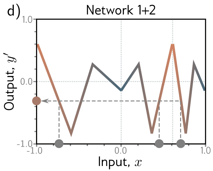
This composed model is also piecewise linear — but with potentially more regions than a shallow network of six hidden units.

The counting argument

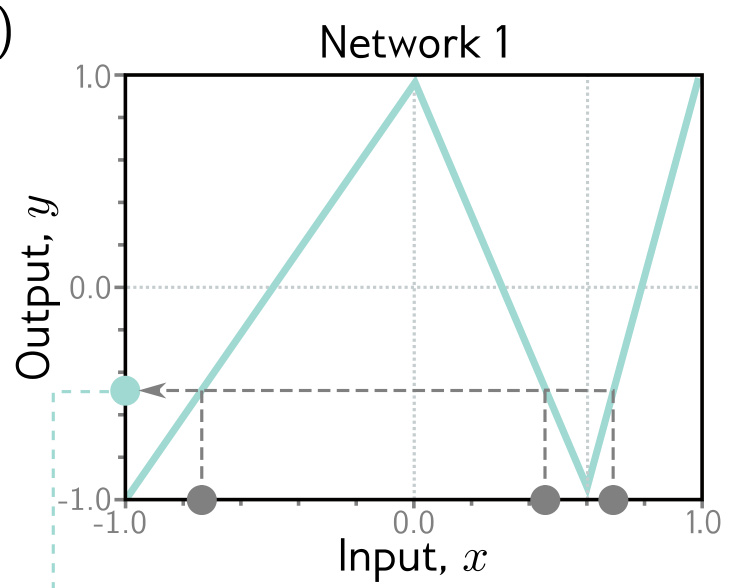
Network 1: \(x \mapsto y\)

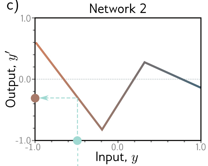
Network 2: \(y \mapsto y'\)

Composed

Three ranges of \(x\) give the same \(y\), so network 2 is applied three times — nine regions, flipped and rescaled.

The same principle holds in higher dimensions. Composing the two-input, three-unit network of the previous section — whose output has seven linear regions, one of them flat — with a second network of two hidden units divides each of the six non-flat regions in two, for thirteen regions in total.

Six units, arranged two ways

Shallow: 6 units, one layer

One joint per unit, so \(6 + 1 = 7\) regions.

Deep: 3 units, then 3 units

The second layer’s function repeats on each fold: 9 regions.

The same six units. The arrangement, not the count, decides how many regions they buy.

This is the point of the whole section. Depth is not more capacity in the sense of more parameters — it is the same budget spent so that regions multiply rather than add.

Deep networks in matrix notation

Two hidden layers, written out

\[h_d = a[\theta_{d0} + \theta_{d1}x],\]

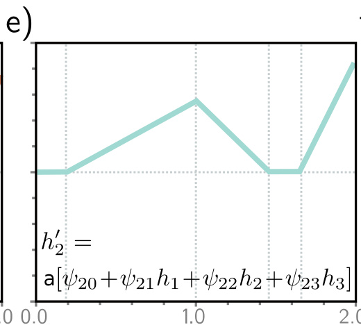
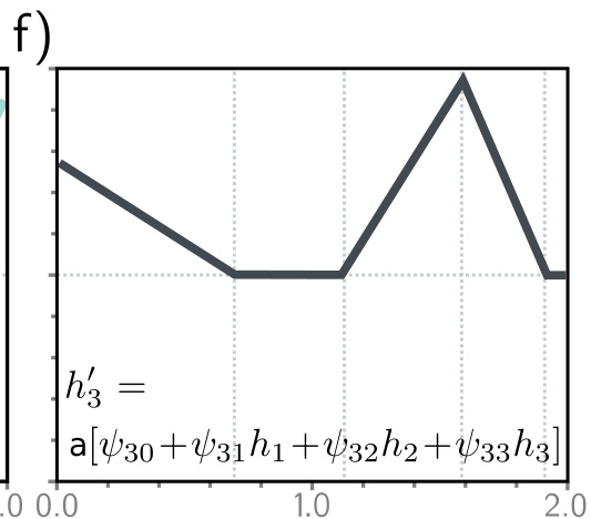
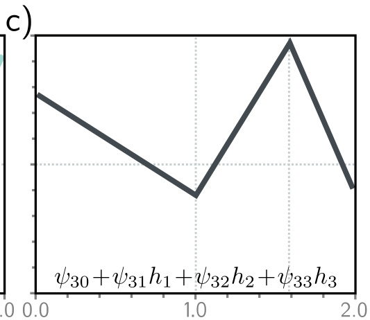
\[h'_d = a[\psi_{d0} + \psi_{d1}h_1 + \psi_{d2}h_2 + \psi_{d3}h_3],\]

\[y' = \phi'_0 + \phi'_1 h'_1 + \phi'_2 h'_2 + \phi'_3 h'_3.\]

The construction has four steps: linear functions of the input through a ReLU; new linear functions of those units; a second ReLU, clipping them and adding new joints; a linear combination of the second layer.

After the second step the object is a shallow network with three outputs, so the three piecewise linear functions have their joints in the same places. It is the second ReLU that breaks that and adds joints of its own.

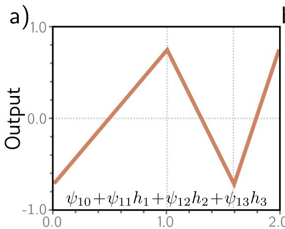
Stage 1: pre-activations at layer two

Already piecewise linear, and all three share their joints.

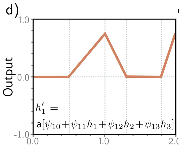
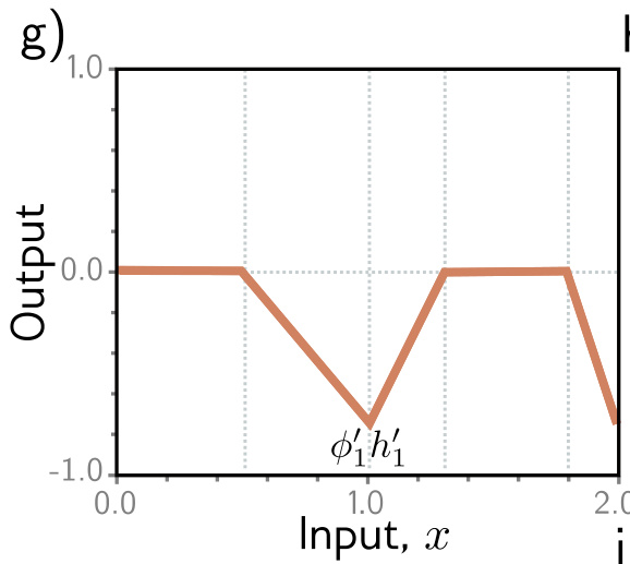
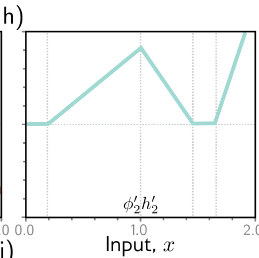
Stage 2: the second ReLU adds joints

Clipping breaks the shared pattern — each unit gains joints of its own.

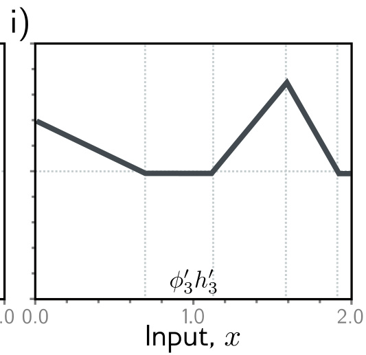
Stage 3: weight each one

Scaled by \(\phi'_1, \phi'_2, \phi'_3\).

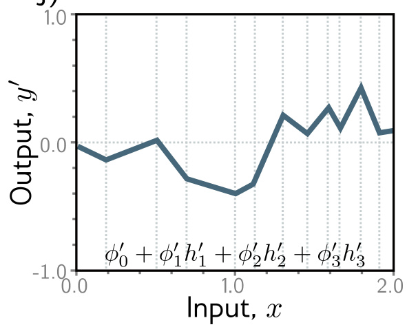
Stage 4: sum, with the offset

• Far more regions than one hidden layer gives
• Two ReLUs, two rounds of joints
• \(\phi'_0\) sets the height

Each layer can be read either as folding the input space or as creating new functions which are clipped and recombined. The first view emphasises the dependencies between regions; the second emphasises how clipping creates new joints. Both are partial. What the network is, without metaphor, is an equation relating input to output.

The general formulation

Layer by layer

\[\begin{aligned} \mathbf{h}_1 &= \mathbf{a}[\boldsymbol{\beta}_0 + \boldsymbol{\Omega}_0\mathbf{x}] \\ \mathbf{h}_{k} &= \mathbf{a}[\boldsymbol{\beta}_{k-1} + \boldsymbol{\Omega}_{k-1}\mathbf{h}_{k-1}] \\ \mathbf{y} &= \boldsymbol{\beta}_K + \boldsymbol{\Omega}_K\mathbf{h}_K \end{aligned}\]

Reading it

• \(\mathbf{a}[\bullet]\) acts element by element
• \(\boldsymbol{\Omega}_k\) are weights, \(\boldsymbol{\beta}_k\) biases
• \(\boldsymbol{\phi} = \{\boldsymbol{\beta}_k, \boldsymbol{\Omega}_k\}_{k=0}^{K}\)

Every deep network is this: affine maps alternating with an element-wise nonlinearity.

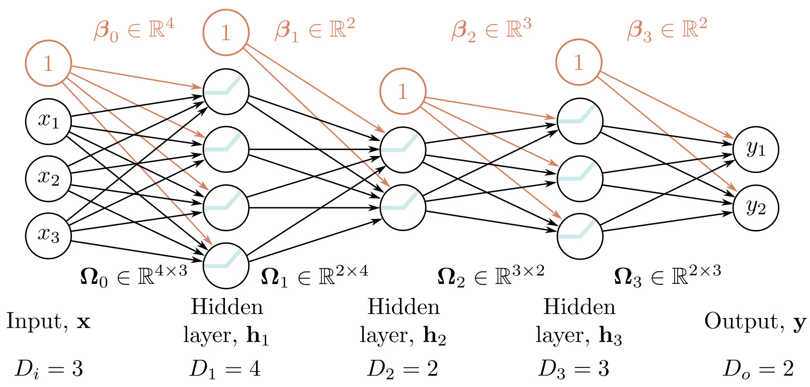
The layer widths force the shapes

\(D_i = 3\), \(D_o = 2\), widths \(4, 2, 3\)

Layer \(k\) has \(D_k\) units, so:

• \(\boldsymbol{\beta}_{k-1}\) has size \(D_k\)
• \(\boldsymbol{\Omega}_0\) is \(D_1 \times D_i\)
• \(\boldsymbol{\Omega}_K\) is \(D_o \times D_K\)
• the rest are \(D_{k+1} \times D_k\)

Nothing is chosen here — the widths fix every shape.

For that network the weight matrices contribute \(4 \times 3 + 2 \times 4 + 3 \times 2 + 2 \times 3 = 32\) parameters and the bias vectors contribute \(4 + 2 + 3 + 2 = 11\), for 43 in total. Hidden layers need not have equal widths, and none of these three does.

Parameters and hyperparameters

Parameters

\(\boldsymbol{\phi} = \{\boldsymbol{\beta}_k, \boldsymbol{\Omega}_k\}\) — the weights and biases, learned by minimizing a loss.

Hyperparameters

The number of layers \(K\) and the widths \(D_1, \ldots, D_K\) — chosen before the parameters are learned.

Fixed hyperparameters give a family of functions; taking them into account as well, a network is a family of families of functions.

Conflating the two is the standard error at this point. The number of hidden units in each layer is the width, the number of hidden layers the depth, and the total number of hidden units a measure of capacity.

Representability is not the interesting question

• A deep network can represent two composed shallow networks
• If the second computes the identity, it is a shallow network
• So it inherits universal approximation

Both families approximate anything. The question is at what cost.

Shallow against deep

Three comparisons

Approximation power alone does not decide between the families.

• Linear regions per parameter
• Large structured inputs
• Training and generalization

The first is theoretical; the last two are empirical.

Linear regions per parameter

Shallow, \(D > 2\) units

up to \(D + 1\) regions on \(3D + 1\) parameters

Deep, \(K\) layers of \(D > 2\) units

up to \((D+1)^K\) regions on \(3D + 1 + (K-1)D(D+1)\) parameters

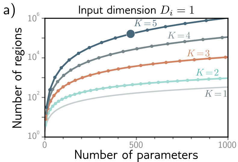
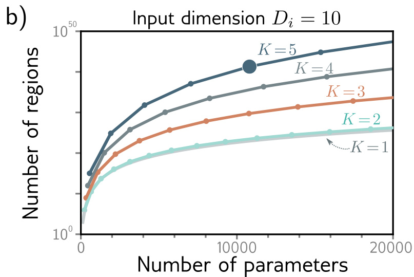
It is the difference between adding and multiplying. \(K = 5\) layers of \(D = 10\) units: \(471\) parameters, \(161{,}051\) regions — against roughly \(150\) for a shallow network on the same budget.

The effect is magnified as input dimension grows. With \(D_i = 10\), a model with \(K = 5\) layers of \(D = 50\) hidden units has \(10{,}801\) parameters and can create more than \(10^{40}\) linear regions.

The growth, plotted

Input dimension \(D_i = 1\), depths \(K = 1\) to \(5\).

The same at \(D_i = 10\).

At a fixed parameter budget, deeper networks produce more regions.

Large structured inputs

• An image is around \(10^6\) pixels
• Fully connected, the parameter count is prohibitive
• And the same object should not be relearned at every position

Process local regions in parallel, then integrate over larger ones — which needs multiple layers.

Training and generalization

• Moderately deep networks are usually easier to train than shallow ones.
• Deep networks appear to generalize to new data better than shallow ones.

Both are reported as observations, not as results. Neither is well understood.

One conjecture for the first is that over-parameterized deep models — those with more parameters than training examples — possess a large family of roughly equivalent solutions that are easy to find. As more hidden layers are added, training becomes more difficult again, and methods for mitigating that are the subject of later material.

On the second: in practice the best results for most tasks have been achieved using networks with tens or hundreds of layers.

What this unit establishes

The template, and the three families

• A parameterized function, learned from examples
• Training minimizes a loss over the training set
• Test data judges it: underfitting against overfitting
• Linear regression shows the workflow, drawable

Two parameters make the loss surface a visible object rather than an abstraction, which is what makes the linear regression example worth the space it takes.

Shallow networks

• One hidden layer; one joint per unit
• Universal approximation: existence, no bound on width
• Multivariate: widen the matrices, joints become hyperplanes
• Without a nonlinearity, the layers collapse to one linear map

Deep networks

• Exponentially more regions per parameter, by folding
• The regions are dependent — the count overstates flexibility
• Alternating matrix multiplies, biases, nonlinearities
• Depth and width are fixed before training
• Depth wins on efficiency, training, and structured inputs

Where next

Two things were asserted rather than derived

The least-squares loss was introduced by stipulation, and descend the loss surface was left without an algorithm behind it.

Training Models supplies both — losses derived from maximum likelihood, and the optimizers that minimize them: stochastic gradient descent, momentum, Adam, together with backpropagation.

Deriving losses from maximum likelihood makes least-squares and cross-entropy follow from a single principle rather than from separate conventions. Backpropagation is the algorithm that computes the gradients the networks of this unit require.