Lecture notes — Training Models
ver. 1.2.0, training_models
ver. 1.2.0 · 2026-09-02 08:29:05
Where this fits
The previous unit, Preliminaries to Machine Learning, built shallow and deep networks and wrote a \(K\)-layer network compactly as \(h_{k+1} = a[\beta_k + \Omega_k h_k]\). It asserted the least-squares loss for real-valued targets, and it described training as a search over the parameter space without giving an algorithm for the search.
Two gaps remain. There is no justified loss for outputs that are not real numbers, and there is no procedure that produces the parameters, no way to compute the derivatives such a procedure needs, and no measurement that separates a well-fitted model from one that has memorised its training set.
This unit closes both. Losses are derived from maximum likelihood; the derived loss is minimised by stochastic gradient descent and its variants; the gradients those variants consume are computed by backpropagation from parameters initialised so that signals survive depth; the result is measured on held-out data and decomposed into its sources; and the gap that measurement exposes is attacked by regularization.
Learning outcomes
derive-loss-from-likelihood— Derive a loss function by treating a network as predicting the parameters of a distribution over outputs.apply-loss-recipe— Apply the four-step recipe to build a loss for a given output type.build-classification-losses— Build binary and multiclass classification losses and relate them to cross-entropy.run-gradient-descent— Run gradient descent on a loss surface and predict where it will fail.use-stochastic-gradients— Explain why stochastic gradient descent on minibatches is both cheaper and better behaved.apply-momentum-and-adam— Apply momentum and Adam, and say what problem each one fixes.set-training-hyperparameters— Choose learning rate, batch size, and schedule, and know which choices matter most.compute-gradients-by-backprop— Compute the gradients of a deep network’s loss by backpropagation.initialize-parameters— Initialize weights so activations and gradients neither vanish nor explode.decompose-test-error— Decompose test error into noise, bias, and variance, and diagnose which dominates.explain-double-descent— Explain double descent and why over-parameterized networks defy the classical bias-variance curve.select-hyperparameters— Use a validation split to select hyperparameters without contaminating the test set.apply-explicit-regularization— Add an explicit regularization term and read it as a prior over parameters.recognize-implicit-regularization— Recognize that gradient descent and SGD regularize on their own.apply-regularization-heuristics— Apply practical regularizers — early stopping, dropout, ensembling, augmentation, transfer learning.
Concepts introduced
- Loss function — a function \(L[\phi]\) returning one number that describes the mismatch between the model predictions \(f[x_i,\phi]\) and the ground-truth outputs \(y_i\).
- Maximum likelihood criterion — choose the parameters that maximise the combined probability of the training outputs under the distributions the model predicts.
- Negative log-likelihood — the log-likelihood multiplied by minus one, which turns maximisation into the minimisation that fitting procedures expect.
- Least squares loss — the sum of squared deviations, which is the negative log-likelihood of a normal distribution whose mean the network predicts.
- Heteroscedastic regression — regression in which the predicted variance is itself a function of the input.
- Binary cross-entropy loss — the negative log-likelihood of a Bernoulli distribution whose parameter is the sigmoid of the network output.
- Multiclass cross-entropy loss — the negative log-likelihood of a categorical distribution whose parameters are the softmax of \(K\) network outputs.
- Cross-entropy and KL divergence equivalence — minimising the KL divergence from the empirical data distribution to the model distribution is minimising negative log-likelihood.
- Gradient descent — repeatedly compute \(\partial L/\partial\phi\) and move the parameters a distance governed by \(\alpha\) in the downhill direction.
- Convexity, local minima, and saddle points — properties of the loss surface that decide whether descent reaches the global minimum, stalls, or terminates elsewhere.
- Stochastic gradient descent — compute the gradient from a random subset of the training pairs rather than from all of them.
- Momentum — replace the current gradient by an exponentially weighted average of the current and past gradients.
- Nesterov accelerated momentum — evaluate the gradient at the point the momentum step is about to reach rather than at the current point.
- Adam — momentum on both the gradient and the squared gradient, with the second used to normalise the first coordinate by coordinate.
- Training algorithm hyperparameters — the optimiser, learning rate and schedule, momentum coefficients and batch size, none of which is learned by the gradient updates.
- Backpropagation — an algorithm computing every parameter derivative at once by traversing the network forward and then backward.
- Forward pass — the sequential evaluation of the network equations, storing every pre-activation and activation.
- Backward pass — the propagation of \(\partial \ell_i/\partial f_k\) from the output back towards the input, reading off parameter derivatives on the way.
- Algorithmic differentiation — the framework implementation of the same idea, in which every module knows its own derivative.
- Vanishing and exploding gradients — the exponential decay or growth of gradient magnitude with depth during the backward pass.
- He initialization — weights drawn from a zero-mean normal with variance \(2/D_h\) and biases set to zero.
- Gradient checkpointing — store activations only at intervals and recompute the missing ones during the backward pass.
- Distributed training — spread one training step across several devices by splitting the batch, the layers, or the individual matrix operations.
- Generalization — the degree to which performance is maintained on a test set the model was not fitted to.
- Noise, bias, and variance decomposition — the additive split of expected least-squares test error into three terms.
- Bias-variance trade-off — for a fixed dataset size, capacity that lowers bias raises variance, so total error is minimised at an intermediate capacity.
- Double descent — test error rises to a peak where the model has just enough capacity to memorise the data, and falls again beyond it.
- Curse of dimensionality — the volume of a high-dimensional input space overwhelms any feasible number of training points.
- Implicit regularization — the preference for some solutions over others exhibited by gradient descent and SGD themselves.
- Hyperparameter optimization — searching a space that is discrete, conditional and non-differentiable by training models and scoring them on validation data.
- Dataset shift — the statistics of deployed data differing from those of the test set, as covariate, prior or concept shift.
- Explicit regularization — an extra term \(\lambda\cdot g[\phi]\) added to the loss to favour certain parameter values.
- L2 regularization and weight decay — penalise \(\sum_j \phi_j^2\), which drives weights smaller and the output function smoother.
- Early stopping — halt training before convergence, at the point of best validation performance.
- Ensembling — average or vote across several trained models so that their independent errors cancel.
- Dropout — clamp a random subset of hidden units to zero at each training iteration.
- Noise injection and label smoothing — perturb inputs, weights or labels during training so that the fitted function is less sharp and less overconfident.
- Bayesian inference in neural networks — treat the parameters as uncertain and predict by an integral weighted by their posterior probability.
- Transfer and multi-task learning — reuse a representation learned on a data-rich secondary task, or learn several tasks at once.
- Self-supervised learning — manufacture the secondary task from unlabelled data, generatively or contrastively.
- Data augmentation — transform each training example in ways that leave its label unchanged.
Maximum likelihood and the negative log-likelihood
Until now the model \(f[x,\phi]\) was taken to compute a prediction \(y\) directly. Understanding Deep Learning shifts perspective and treats the model as computing a conditional probability distribution \(Pr(y|x)\) over possible outputs given the input. The loss then encourages each training output \(y_i\) to have high probability under the distribution computed from the corresponding input \(x_i\).
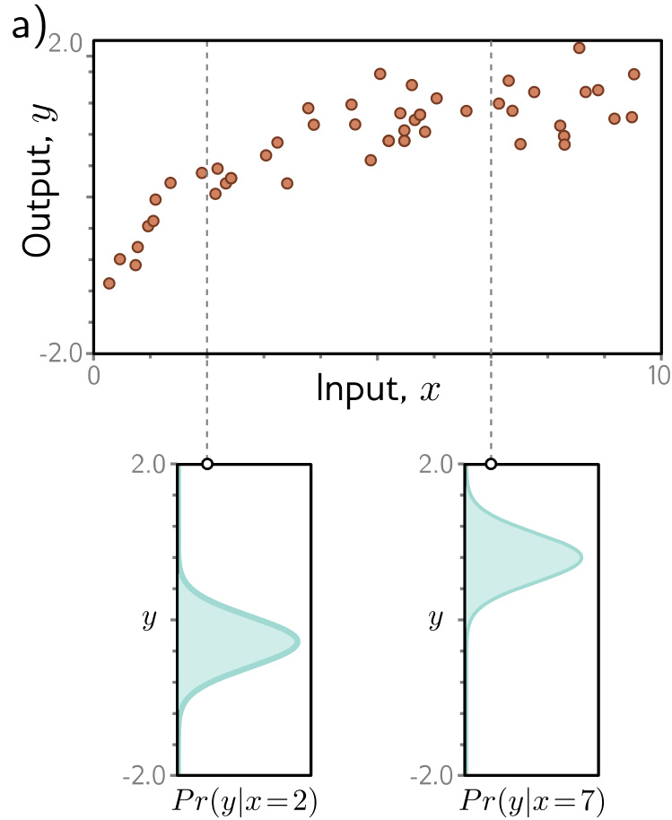
The mechanism is to choose a parametric distribution \(Pr(y|\theta)\) defined on the output domain and have the network compute one or more of the parameters \(\theta\) of that distribution. For \(y \in \mathbb{R}\) the univariate normal distribution has \(\theta = \{\mu, \sigma^2\}\); the model might predict the mean \(\mu\), and the variance \(\sigma^2\) could be treated as an unknown constant.
Each training input now yields its own parameters \(\theta_i = f[x_i,\phi]\), and the maximum likelihood criterion chooses the parameters that maximise the combined probability across all \(I\) training examples:
\[\hat{\phi} = \underset{\phi}{\operatorname{argmax}} \left[ \prod_{i=1}^{I} Pr(y_i|f[x_i,\phi]) \right].\]
Two assumptions are implicit and both are worth naming. The data are identically distributed — the form of the distribution over the outputs is the same for each data point — and the conditional distributions \(Pr(y_i|x_i)\) are independent, so that the total likelihood factorises as \(Pr(y_1,\dots,y_I|x_1,\dots,x_I) = \prod_{i=1}^I Pr(y_i|x_i)\). Together these are the i.i.d. assumption.
The criterion as written is not practical. Each factor \(Pr(y_i|f[x_i,\phi])\) can be small, so a product of many of them can be tiny and difficult to represent in finite-precision arithmetic. Taking the logarithm converts the product into a sum:
\[\hat{\phi} = \underset{\phi}{\operatorname{argmax}} \left[ \sum_{i=1}^{I} \log\big[Pr(y_i|f[x_i,\phi])\big] \right].\]
The two criteria have the same maximiser because the logarithm is strictly monotonically increasing: if \(z > z'\) then \(\log[z] > \log[z']\). Positions of positive slope keep a positive slope after the transform, and the position of the maximum does not move.
Fitting problems are framed by convention as minimisation, so the log-likelihood is multiplied by minus one, giving the negative log-likelihood criterion:
\[\hat{\phi} = \underset{\phi}{\operatorname{argmin}} \left[ -\sum_{i=1}^{I} \log\big[Pr(y_i|f[x_i,\phi])\big] \right] = \underset{\phi}{\operatorname{argmin}}\big[L[\phi]\big].\]
Inference is the separate question of what to return at test time. The network determines a distribution rather than a value, so a point estimate is obtained by returning the maximum of that distribution, \(\hat{y} = \operatorname{argmax}_y [Pr(y|f[x,\hat{\phi}])]\). This is usually expressible through the predicted parameters \(\theta\); for the univariate normal the maximum occurs at the mean \(\mu\).
A conditional probability \(Pr(z|\psi)\) read as a function of \(z\) is a distribution and sums to one. Read as a function of \(\psi\) it is a likelihood and does not generally sum to one.
Learning outcomes
- derive-loss-from-likelihood Derive a loss function by treating a network as predicting the parameters of a distribution over outputs.
Concepts
- maximum-likelihood-criterion the parameters are chosen to maximise the product of the probabilities the model assigns to the observed training outputs, under the i.i.d. assumption
- negative-log-likelihood negating the sum of log probabilities gives a numerically stable loss whose minimum is the maximum likelihood estimate
- loss-function the loss that training minimises is the negative log-likelihood \(L[\phi] = -\sum_i \log[Pr(y_i|f[x_i,\phi])]\)
A recipe for losses, and univariate regression
The framework becomes a procedure that can be applied mechanically. For training data \(\{x_i,y_i\}\):
- Choose a suitable probability distribution \(Pr(y|\theta)\) defined over the domain of the predictions \(y\), with distribution parameters \(\theta\).
- Set the model \(f[x,\phi]\) to predict one or more of these parameters, so \(\theta = f[x,\phi]\) and \(Pr(y|\theta) = Pr(y|f[x,\phi])\).
- Find the network parameters \(\hat{\phi}\) that minimise the negative log-likelihood loss over the training pairs.
- For a new test example \(x\), return either the full distribution \(Pr(y|f[x,\hat{\phi}])\) or the value where it is maximised.
Applied to a single scalar output \(y \in \mathbb{R}\), step one selects the univariate normal, whose density is
\[Pr(y|\mu,\sigma^2) = \frac{1}{\sqrt{2\pi\sigma^2}}\exp\left[-\frac{(y-\mu)^2}{2\sigma^2}\right].\]
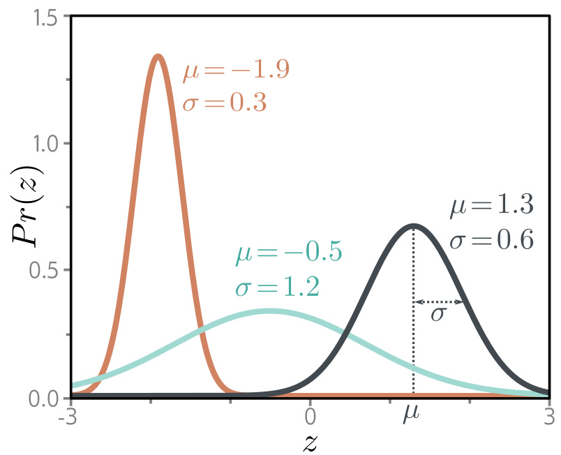
Step two sets \(\mu = f[x,\phi]\). Step three writes the negative log-likelihood and simplifies it:
\[ \begin{aligned} \hat{\phi} &= \underset{\phi}{\operatorname{argmin}}\left[-\sum_{i=1}^{I}\log\left[\frac{1}{\sqrt{2\pi\sigma^2}}\exp\left[-\frac{(y_i-f[x_i,\phi])^2}{2\sigma^2}\right]\right]\right]\\ &= \underset{\phi}{\operatorname{argmin}}\left[-\sum_{i=1}^{I}\left(\log\left[\frac{1}{\sqrt{2\pi\sigma^2}}\right] - \frac{(y_i-f[x_i,\phi])^2}{2\sigma^2}\right)\right]\\ &= \underset{\phi}{\operatorname{argmin}}\left[\sum_{i=1}^{I}(y_i-f[x_i,\phi])^2\right]. \end{aligned} \]
The first term was removed because it does not depend on \(\phi\), and the denominator \(2\sigma^2\) was removed because it is a constant positive scaling factor that does not affect the position of the minimum. What is left is the least squares loss \(L[\phi] = \sum_{i=1}^{I}(y_i - f[x_i,\phi])^2\). Least squares is not a convention; it follows from the assumptions that the predictions are independent and drawn from a normal distribution with mean \(f[x_i,\phi]\).
The two criteria track each other numerically. For the linear model of figure 5.4 a good set of parameters gives \(\sum_i (y_i - f[x_i,\phi])^2 = 0.19\) and \(-\sum_i \log[Pr(y_i|f[x_i,\phi],\sigma^2)] = -6.57\); a bad set gives \(10.22\) and \(497.37\) respectively.
Step four is immediate: the maximum of the univariate normal sits at \(\mu\), which is what the model computed, so \(\hat{y} = f[x,\hat{\phi}]\).
Estimating the variance
Equation 5.11 does not depend on \(\sigma^2\), but nothing prevents treating \(\sigma^2\) as a learned parameter and minimising the full Gaussian negative log-likelihood over both:
\[\hat{\phi},\hat{\sigma}^2 = \underset{\phi,\sigma^2}{\operatorname{argmin}}\left[-\sum_{i=1}^{I}\log\left[\frac{1}{\sqrt{2\pi\sigma^2}}\exp\left[-\frac{(y_i-f[x_i,\phi])^2}{2\sigma^2}\right]\right]\right].\]
At inference the mean \(\mu = f[x,\hat{\phi}]\) is the prediction and \(\hat{\sigma}^2\) quantifies the uncertainty in it.
Heteroscedastic regression
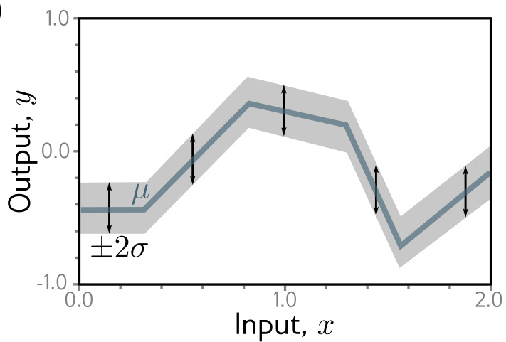
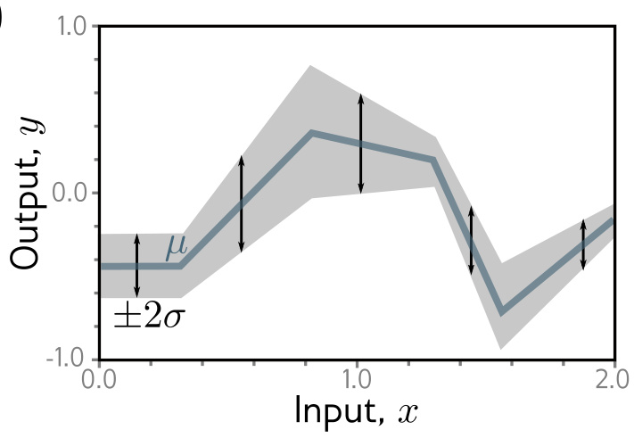
The model above assumes the variance of the data is constant everywhere, which is termed homoscedastic. When uncertainty varies as a function of the input the data are heteroscedastic, and the network is given two outputs: \(f_1[x,\phi]\) predicts the mean and \(f_2[x,\phi]\) predicts the variance. A variance must be positive and a network output cannot be guaranteed to be, so the second output is passed through a function mapping an arbitrary value to a positive one. Squaring is a suitable choice:
\[\mu = f_1[x,\phi], \qquad \sigma^2 = f_2[x,\phi]^2,\]
which gives the loss
\[\hat{\phi} = \underset{\phi}{\operatorname{argmin}}\left[-\sum_{i=1}^{I}\left(\log\left[\frac{1}{\sqrt{2\pi f_2[x_i,\phi]^2}}\right] - \frac{(y_i - f_1[x_i,\phi])^2}{2f_2[x_i,\phi]^2}\right)\right].\]
Learning outcomes
- apply-loss-recipe Apply the four-step recipe to build a loss for a given output type.
- derive-loss-from-likelihood Derive a loss function by treating a network as predicting the parameters of a distribution over outputs.
Concepts
- least-squares-loss discarding the \(\phi\)-independent constant and the positive scaling factor from the Gaussian negative log-likelihood leaves the sum of squared deviations
- loss-function a regression loss is a consequence of a distributional assumption rather than a choice made in advance
- negative-log-likelihood the Gaussian negative log-likelihood also supports a learned variance and an input-dependent variance
- heteroscedastic-regression a second network output passed through a positivity transform makes the predicted variance a function of the input
Classification losses and cross-entropy
Nothing new is invented for classification; only step one of the recipe changes.
In binary classification the goal is to assign the data \(x\) to one of two discrete classes \(y \in \{0,1\}\), where \(y\) is termed a label. Predicting whether a restaurant review is positive from text, or whether a tumour is present from an MRI scan, are instances. The distribution over \(\{0,1\}\) is the Bernoulli, with a single parameter \(\lambda \in [0,1]\) representing the probability that \(y\) takes the value one:
\[Pr(y|\lambda) = (1-\lambda)^{1-y}\cdot\lambda^{y}.\]
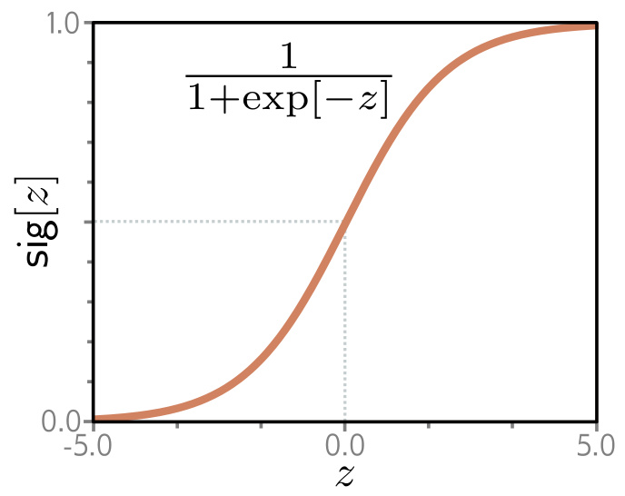
Because \(\lambda\) must lie in \([0,1]\) and a network output cannot be guaranteed to, the output is passed through the logistic sigmoid
\[\operatorname{sig}[z] = \frac{1}{1+\exp[-z]},\]
so \(\lambda = \operatorname{sig}[f[x,\phi]]\). Minimising the negative log-likelihood of the training set gives the binary cross-entropy loss
\[L[\phi] = \sum_{i=1}^{I} -(1-y_i)\log\big[1-\operatorname{sig}[f[x_i,\phi]]\big] - y_i \log\big[\operatorname{sig}[f[x_i,\phi]]\big].\]
At inference \(\operatorname{sig}[f[x,\phi]]\) is the probability that \(y=1\), so a point estimate sets \(y=1\) if \(\lambda > 0.5\) and \(y=0\) otherwise.
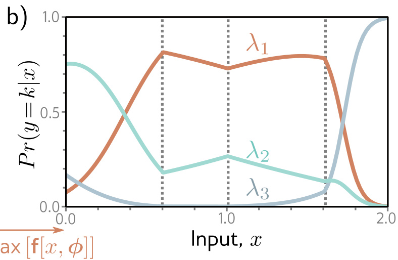
In multiclass classification the input is assigned to one of \(K > 2\) classes, \(y \in \{1,2,\dots,K\}\) — which of \(K=10\) digits appears in an image, or which of \(K\) possible words follows an incomplete sentence. The categorical distribution on this domain has \(K\) parameters with \(Pr(y=k) = \lambda_k\), each constrained to \([0,1]\) and collectively summing to one. A network with \(K\) outputs computes them through the softmax function
\[\operatorname{softmax}_k[z] = \frac{\exp[z_k]}{\sum_{k'=1}^{K}\exp[z_{k'}]},\]
where the exponentials ensure positivity and the denominator ensures the \(K\) numbers sum to one. The negative log-likelihood of the training data is the multiclass cross-entropy loss
\[L[\phi] = -\sum_{i=1}^{I}\left(f_{y_i}[x_i,\phi] - \log\left[\sum_{k'=1}^{K}\exp\big[f_{k'}[x_i,\phi]\big]\right]\right),\]
where \(f_{y_i}[x_i,\phi]\) and \(f_{k'}[x_i,\phi]\) denote the \(y_i^{th}\) and \(k'^{th}\) outputs of the network. The point estimate is the most probable category, \(\hat{y} = \operatorname{argmax}_k[Pr(y=k|f[x,\hat{\phi}])]\).
Multiple outputs
When the target \(y\) is a vector it is more usual to treat each prediction as independent than to define a multivariate distribution, so that
\[Pr(y|f[x,\phi]) = \prod_d Pr(y_d|f_d[x,\phi]),\]
where \(f_d[x,\phi]\) is the \(d^{th}\) set of network outputs describing the parameters of the distribution over \(y_d\). Under the negative log-likelihood the product becomes a sum of terms,
\[L[\phi] = -\sum_{i=1}^{I}\sum_d \log\big[Pr(y_{id}|f_d[x_i,\phi])\big],\]
which is what lets one network mix output types: predicting wind direction and strength together uses a von Mises distribution for the direction and an exponential distribution for the strength, and the two negative log-likelihoods add.
Cross-entropy
The term cross-entropy loss is commonplace, and it names the same objective. Cross-entropy seeks parameters minimising the distance between the empirical distribution \(q(y)\) of the observed data and a model distribution \(Pr(y|\theta)\), measured by the Kullback-Leibler divergence
\[D_{KL}[q||p] = \int_{-\infty}^{\infty} q(z)\log[q(z)]dz - \int_{-\infty}^{\infty} q(z)\log[p(z)]dz.\]
The empirical distribution at the observed points \(\{y_i\}_{i=1}^I\) is a weighted sum of point masses, \(q(y) = \frac{1}{I}\sum_{i=1}^{I}\delta[y-y_i]\), where \(\delta[\bullet]\) is the Dirac delta function. The first term of the divergence has no dependence on \(\theta\) and disappears; the second is the cross-entropy. Substituting the definition of \(q(y)\) and eliminating the constant factor \(1/I\) leaves
\[\hat{\theta} = \underset{\theta}{\operatorname{argmin}}\left[-\sum_{i=1}^{I}\log\big[Pr(y_i|\theta)\big]\right],\]
and with \(\theta\) computed by the model this is precisely the negative log-likelihood criterion. The two criteria are equivalent.
Learning outcomes
- build-classification-losses Build binary and multiclass classification losses and relate them to cross-entropy.
- apply-loss-recipe Apply the four-step recipe to build a loss for a given output type.
Concepts
- binary-cross-entropy a Bernoulli output whose parameter is the sigmoid of the network output yields the binary cross-entropy loss
- multiclass-cross-entropy a categorical output whose parameters are the softmax of \(K\) network outputs yields the multiclass cross-entropy loss
- cross-entropy-kl-divergence minimising the KL divergence from the empirical distribution of point masses to the model distribution reduces exactly to minimising negative log-likelihood
Gradient descent and loss surfaces
With a loss in hand, fitting is the optimisation problem \(\hat{\phi} = \operatorname{argmin}_\phi[L[\phi]]\). The standard methods for neural networks are iterative: initialise the parameters heuristically, then adjust them repeatedly so that the loss decreases. The simplest such method is gradient descent, which starts with \(\phi = [\phi_0,\phi_1,\dots,\phi_N]^T\) and iterates two steps.
Step 1 computes the derivatives of the loss with respect to the parameters, \(\partial L/\partial\phi = [\partial L/\partial\phi_0, \dots, \partial L/\partial\phi_N]^T\).
This vector points in the uphill direction of the loss function.
Step 2 updates the parameters by \(\phi \longleftarrow \phi - \alpha\cdot\frac{\partial L}{\partial\phi}\), where the positive scalar \(\alpha\) determines the magnitude of the change.
The negative sign moves a small distance \(\alpha\) downhill. The parameter \(\alpha\) may be fixed — then it is called the learning rate — or chosen by a line search that tries several values of \(\alpha\) and keeps the one decreasing the loss most.
At a minimum the surface is flat, so the gradient is zero and the parameters stop changing. In practice the gradient magnitude is monitored and the algorithm terminated when it becomes too small.
For 1D linear regression \(y = \phi_0 + \phi_1 x\) with the least squares loss \(L[\phi] = \sum_{i=1}^{I}(\phi_0 + \phi_1 x_i - y_i)^2\), the gradient decomposes into a sum of per-example contributions \(\partial L/\partial\phi = \sum_i \partial\ell_i/\partial\phi\) with
\[\frac{\partial \ell_i}{\partial\phi} = \begin{bmatrix} 2(\phi_0 + \phi_1 x_i - y_i)\\ 2x_i(\phi_0+\phi_1 x_i - y_i)\end{bmatrix}.\]
Four line-search iterations on a training set of \(I=12\) pairs already bring the fit close to the minimum.
Loss surfaces for linear regression always have a single well-defined global minimum. More formally they are convex: every chord — the line segment between two points on the surface — lies above the function and does not intersect it. Convexity implies that wherever the parameters are initialised, walking downhill is bound to reach the minimum, so the training procedure cannot fail.
Loss functions for most nonlinear models, shallow and deep networks included, are non-convex. Visualising a network loss surface is difficult because of the number of parameters, so Understanding Deep Learning studies a two-parameter nonlinear model, the Gabor model
\[f[x,\phi] = \sin[\phi_0 + 0.06\cdot\phi_1 x]\cdot\exp\left(-\frac{(\phi_0+0.06\cdot\phi_1 x)^2}{32.0}\right),\]
a sinusoid whose amplitude decreases away from its centre. Its training set contains 28 pairs sampled uniformly over \(x_i \in [-15,15]\) from a Gabor model with \(\phi = [0.0, 16.6]^T\) plus normally distributed noise.
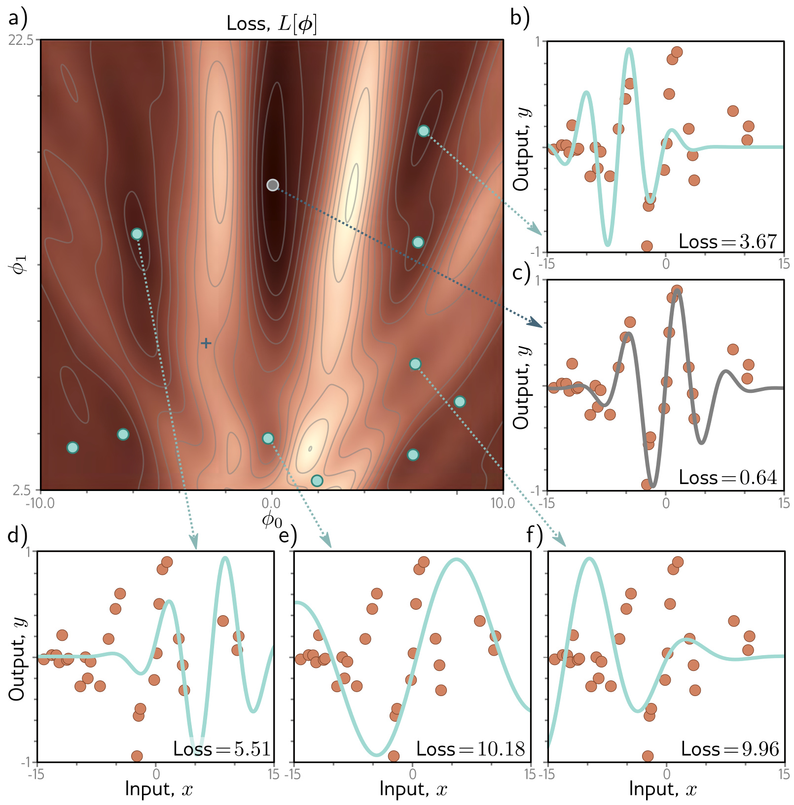
The surface names the obstacles precisely.
- Local minima are points where the gradient is zero and the loss increases in every direction, but which are not the overall minimum of the function. Their associated models have losses of 3.67, 5.51, 9.96 and 10.18 against the global minimum’s 0.64, and at each of them no small parameter change decreases the loss.
- Saddle points are points where the gradient is zero but the function increases in some directions and decreases in others. Descent can escape one by moving downhill if it is not exactly at the point, but the surface nearby is flat, so an algorithm that terminates on a small gradient may erroneously stop there.
Starting from a random position and descending gives no guarantee of arriving at the global minimum, and no way of knowing whether a better solution exists elsewhere.
Learning outcomes
- run-gradient-descent Run gradient descent on a loss surface and predict where it will fail.
Concepts
- gradient-descent the update \(\phi \leftarrow \phi - \alpha\,\partial L/\partial\phi\) moves downhill by a distance set by a fixed learning rate or by a line search
- convexity-and-local-minima a convex surface guarantees that descent reaches the global minimum, while the non-convex surfaces of nonlinear models hold local minima and saddle points that trap or stall it
Stochastic gradient descent
The Gabor model has two parameters, so its global minimum could be found by searching the parameter space exhaustively or by restarting descent from many positions. Neural networks can have millions of parameters, and neither approach is practical. The destination of a gradient descent run is determined entirely by its starting point.
Stochastic gradient descent adds noise to the gradient at each step. At each iteration the algorithm chooses a random subset of the training data, known as a minibatch or batch, and computes the gradient from those examples alone:
\[\phi_{t+1} \longleftarrow \phi_t - \alpha\cdot\sum_{i\in\mathcal{B}_t}\frac{\partial \ell_i[\phi_t]}{\partial\phi},\]
where \(\mathcal{B}_t\) contains the indices of the input/output pairs in the current batch. The batches are usually drawn without replacement; the algorithm works through the training examples until it has used all the data, at which point it starts sampling from the full dataset again. A single pass through the entire training dataset is an epoch. A batch may be as small as a single example or as large as the whole dataset, and the latter case is full-batch gradient descent, identical to regular gradient descent.
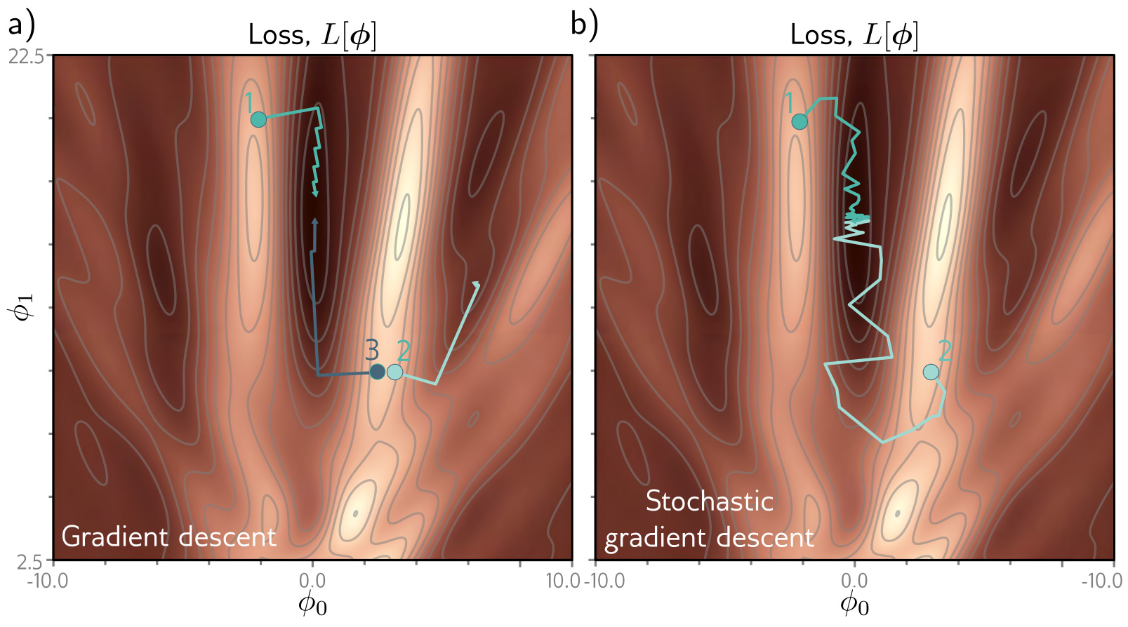
The update still moves downhill on average, but at any given iteration the chosen direction is not the steepest descent direction and need not be downhill at all with respect to the total loss. That is the point: it makes moving temporarily uphill possible, and hence jumping from one valley of the loss function to another.
An alternative reading is that SGD computes the gradient of a different loss function at each iteration, because the loss depends on both the model and the data. In this view SGD performs deterministic gradient descent on a constantly changing loss surface, and a point that is a minimum or a saddle for one batch usually is not for the next. Despite the variability, the expected loss and expected gradients at any point remain the same as for gradient descent.
The properties that follow are these.
- The updates tend to be sensible even when they are not optimal, since each step still improves the fit to a subset of the data.
- Drawing examples without replacement and iterating through the dataset makes all training examples contribute equally.
- Computing the gradient from a subset is computationally less expensive than computing it from the whole training set.
- The algorithm can in principle escape local minima, and it reduces the chance of getting stuck near saddle points, since at least some possible batches are likely to have a significant gradient there.
- There is evidence that SGD finds parameters that generalize well to new data in practice.
SGD does not necessarily converge in the traditional sense. The hope is that near the global minimum all the data points will be well described by the model, so the gradient will be small whichever batch is chosen and the parameters will cease to change much. In practice SGD is applied with a learning rate schedule: \(\alpha\) starts at a high value and is decreased by a constant factor every \(N\) epochs. Early in training the algorithm should explore the parameter space, jumping from valley to valley to find a sensible region; later it is roughly in the right place and is concerned with fine-tuning, so \(\alpha\) is decreased to make smaller changes.
Learning outcomes
- use-stochastic-gradients Explain why stochastic gradient descent on minibatches is both cheaper and better behaved.
Concepts
- stochastic-gradient-descent the gradient is computed from a random minibatch drawn without replacement, which lowers the cost per iteration and lets the trajectory move uphill on the total loss
- convexity-and-local-minima because each batch defines a different loss surface, a point that is a local minimum or saddle for one batch is usually neither for the next
- training-hyperparameters batch size and the schedule that decays the learning rate every \(N\) epochs are decided before training, not learned during it
Momentum and Adam
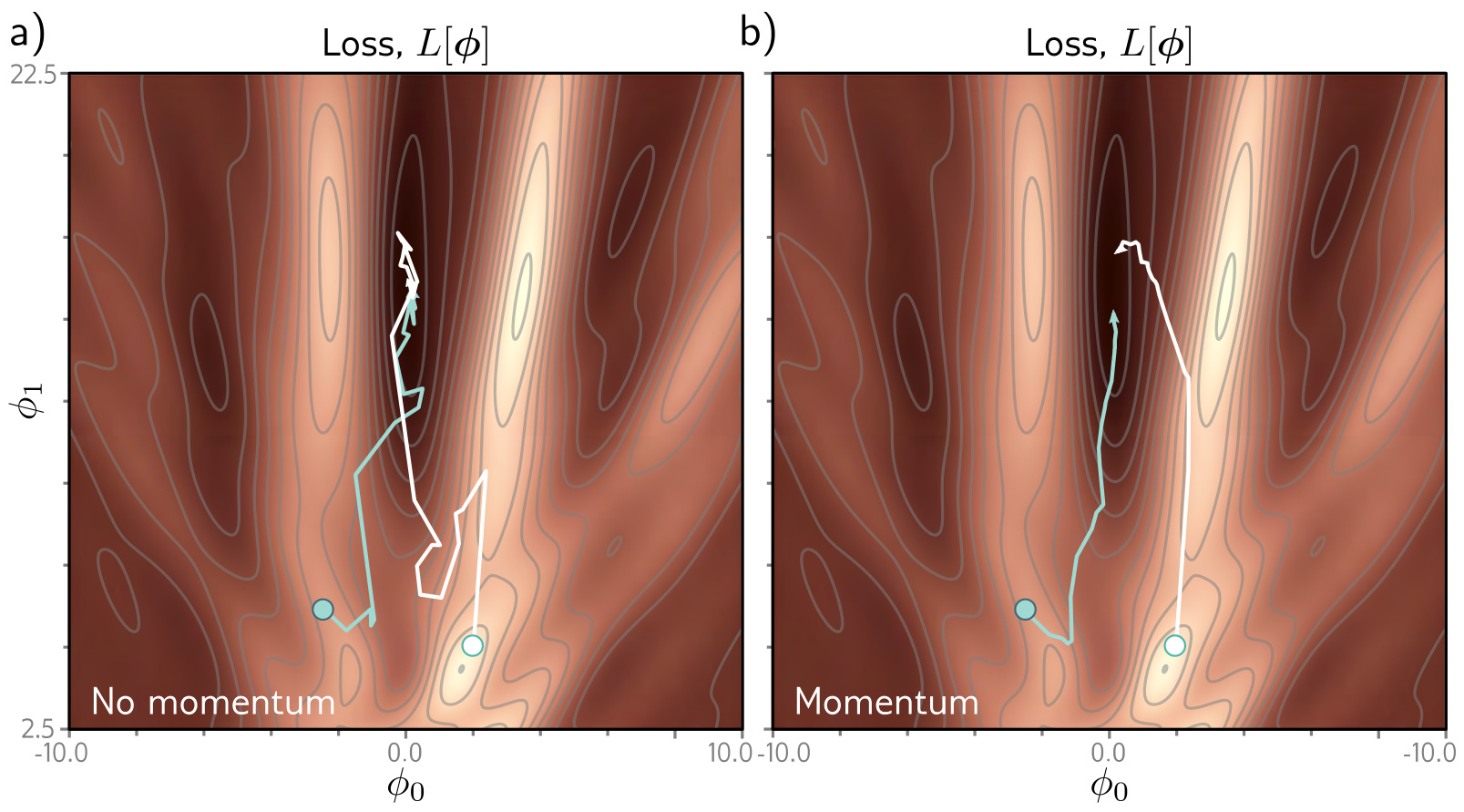
A common modification to SGD is a momentum term, which updates the parameters with a weighted combination of the gradient computed from the current batch and the direction moved in the previous step:
\[ \begin{aligned} m_{t+1} &\leftarrow \beta\cdot m_t + (1-\beta)\sum_{i\in\mathcal{B}_t}\frac{\partial \ell_i[\phi_t]}{\partial\phi}\\ \phi_{t+1} &\leftarrow \phi_t - \alpha\cdot m_{t+1}, \end{aligned} \]
where \(m_t\) is the momentum driving the update at iteration \(t\), \(\beta \in [0,1)\) controls the degree to which the gradient is smoothed over time, and \(\alpha\) is the learning rate. The recursion makes the step an infinite weighted sum of all previous gradients, with weights shrinking as one moves back in time. The effective learning rate increases when those gradients are aligned over multiple iterations and decreases when the gradient direction changes repeatedly, because the terms in the sum cancel. The overall effect is a smoother trajectory and reduced oscillatory behaviour in valleys.
Nesterov accelerated momentum treats the momentum term as a coarse prediction of where the algorithm will move next, and computes the gradients at that predicted point instead of the current one:
\[ \begin{aligned} m_{t+1} &\leftarrow \beta\cdot m_t + (1-\beta)\sum_{i\in\mathcal{B}_t}\frac{\partial \ell_i[\phi_t - \alpha\beta\cdot m_t]}{\partial\phi}\\ \phi_{t+1} &\leftarrow \phi_t - \alpha\cdot m_{t+1}. \end{aligned} \]
The gradient term now corrects the path that momentum alone would take.
Adam
Momentum does not address a separate defect of a fixed step size: it makes large adjustments to parameters with large gradients, where more caution might be warranted, and small adjustments to parameters with small gradients, where further exploration might be warranted. When the surface is much steeper in one direction than another, a learning rate that makes good progress in the shallow direction overshoots and becomes unstable in the steep one, while one that is stable in the steep direction takes a long time in the shallow one.
A straightforward response is to normalise the gradients so that a fixed distance is moved in each direction. Measuring the gradient \(m_{t+1}\) and the pointwise squared gradient \(v_{t+1}\),
\[m_{t+1} \leftarrow \frac{\partial L[\phi_t]}{\partial\phi}, \qquad v_{t+1} \leftarrow \left(\frac{\partial L[\phi_t]}{\partial\phi}\right)^2,\]
and applying \(\phi_{t+1} \leftarrow \phi_t - \alpha\cdot\frac{m_{t+1}}{\sqrt{v_{t+1}}+\epsilon}\) — with the square root and division both pointwise and \(\epsilon\) a small constant preventing division by zero — leaves only the sign in each coordinate. The algorithm then moves a fixed distance \(\alpha\) along each coordinate in whichever direction is downhill. It makes good progress in both directions but will not converge unless it happens to land exactly at the minimum; instead it bounces back and forth around it.
Adaptive moment estimation, or Adam, adds momentum to both estimates:
\[m_{t+1} \leftarrow \beta\cdot m_t + (1-\beta)\frac{\partial L[\phi_t]}{\partial\phi}, \qquad v_{t+1} \leftarrow \gamma\cdot v_t + (1-\gamma)\left(\frac{\partial L[\phi_t]}{\partial\phi}\right)^2,\]
where \(\beta\) and \(\gamma\) are the momentum coefficients for the two statistics. Using momentum is equivalent to taking a weighted average over the history of each statistic, and at the start of the procedure all the previous measurements are effectively zero, which makes the estimates unrealistically small. The statistics are therefore modified by
\[\tilde{m}_{t+1} \leftarrow \frac{m_{t+1}}{1-\beta^{t+1}}, \qquad \tilde{v}_{t+1} \leftarrow \frac{v_{t+1}}{1-\gamma^{t+1}},\]
and the update becomes \(\phi_{t+1} \leftarrow \phi_t - \alpha\cdot\frac{\tilde{m}_{t+1}}{\sqrt{\tilde{v}_{t+1}}+\epsilon}\). Since \(\beta\) and \(\gamma\) lie in \([0,1)\), the terms with exponent \(t+1\) shrink at each step, the denominators approach one, and the correction has a diminishing effect.
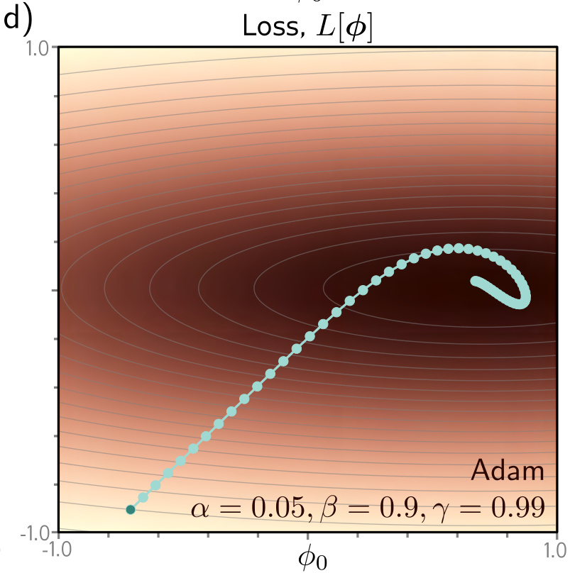
In practice Adam is used in a stochastic setting, with both the gradient and its square computed from minibatches, so the trajectory is noisy. Gradient magnitudes in a neural network depend on the depth of the parameter in the network; Adam compensates for this tendency and balances changes across the different layers. It also has the practical advantage of being less sensitive to the initial learning rate, so it does not need complex learning rate schedules.
Learning outcomes
- apply-momentum-and-adam Apply momentum and Adam, and say what problem each one fixes.
- run-gradient-descent Run gradient descent on a loss surface and predict where it will fail.
Concepts
- momentum an exponentially weighted average of past gradients accumulates along consistent directions and cancels across oscillating ones
- nesterov-accelerated-momentum evaluating the gradient at \(\phi_t - \alpha\beta m_t\) corrects the path that the momentum step alone would take
- adam-optimizer dividing a momentum estimate of the gradient by the square root of a momentum estimate of its square equalises step sizes across coordinates, with bias corrections for the early iterations
- training-hyperparameters the momentum coefficients \(\beta\) and \(\gamma\), the constant \(\epsilon\) and the learning rate \(\alpha\) are all set by hand, and Adam reduces the sensitivity to the last of them
Hyperparameters of the training algorithm
The choices of learning algorithm, batch size, learning rate schedule, and momentum coefficients are all hyperparameters of the training algorithm. They directly affect the final model performance but are distinct from the model parameters \(\phi\): the gradient updates learn \(\phi\), and nothing in the training loop learns the hyperparameters.
Choosing them is more art than science. The usual practice is to train many models with different hyperparameters and choose the best one, which is hyperparameter search; the protocol that makes such a comparison honest is the subject of a later section.
One schedule is worth naming beyond the decay described above. Adaptive algorithms base their learning rates on accumulated statistics of the observed gradients, and at the start of training, when there are few samples, those statistics may be very noisy. Learning rate warm-up remedies this by increasing the learning rates gradually over the first few thousand iterations.
The chapter’s summary states the position reached. Model training is the problem of finding parameters \(\phi\) corresponding to the minimum of a loss function \(L[\phi]\). Gradient descent measures how the loss changes when the parameters change slightly, then moves them in the direction that decreases the loss fastest, repeating until convergence. For nonlinear functions the loss may have both local minima, where descent gets trapped, and saddle points, where descent may appear to have converged but has not. SGD mitigates both problems by using a different random subset of the data at each iteration, and is also computationally cheaper per iteration. Momentum makes convergence more efficient. Adam combines momentum with per-coordinate normalization.
These ideas apply to optimizing any model. What remains specific to neural networks is how to compute the gradients the updates consume, and how to initialize the parameters before optimization begins.
Learning outcomes
- set-training-hyperparameters Choose learning rate, batch size, and schedule, and know which choices matter most.
- use-stochastic-gradients Explain why stochastic gradient descent on minibatches is both cheaper and better behaved.
Concepts
- training-hyperparameters the optimiser, learning rate and its schedule, batch size and momentum coefficients are configuration of the training algorithm, chosen by search rather than by gradient
- gradient-descent the iterative measure-then-move framework underlies every optimiser in this unit
- stochastic-gradient-descent minibatch noise is what mitigates local minima and saddle points on non-convex surfaces
- momentum accumulating gradient history is what makes convergence more efficient
- adam-optimizer Adam is the combination of momentum with adaptive per-coordinate scaling
Backpropagation
Every optimiser above assumed the gradients were available. For a network with three hidden layers,
\[ \begin{aligned} h_1 &= a[\beta_0 + \Omega_0 x], & h_2 &= a[\beta_1 + \Omega_1 h_1],\\ h_3 &= a[\beta_2 + \Omega_2 h_2], & f[x,\phi] &= \beta_3 + \Omega_3 h_3, \end{aligned} \]
the parameters are the bias vectors \(\beta_k\) and weight matrices \(\Omega_k\), and the SGD update requires \(\partial\ell_i/\partial\beta_k\) and \(\partial\ell_i/\partial\Omega_k\) for every layer \(k\) and every index \(i\) in the batch. The largest models at the time of writing have around \(10^{12}\) parameters, and these derivatives are needed at every iteration.
Two observations give the shape of the algorithm.
- Observation 1. Each weight multiplies the activation at a source hidden unit and adds the result to a destination hidden unit in the next layer, so the effect of any small change to the weight is amplified or attenuated by the activation at the source unit. The network is therefore run for each data example in the batch and the activations of all the hidden units are stored. This is the forward pass.
- Observation 2. A small change in a bias or weight causes a ripple of changes through the subsequent network, so to know how changing a parameter modifies the loss one also needs to know how changes to every subsequent hidden layer modify their successor. The same quantities are required for parameters in the same or earlier layers, so they can be calculated once and reused — which requires computing them in reverse order. This is the backward pass.
The toy example
The mechanics are clearest on a model with eight scalar parameters and a composition of \(\sin[\bullet]\), \(\exp[\bullet]\) and \(\cos[\bullet]\):
\[f[x,\phi] = \beta_3 + \omega_3\cdot\cos\big[\beta_2 + \omega_2\cdot\exp\big[\beta_1+\omega_1\cdot\sin[\beta_0+\omega_0\cdot x]\big]\big],\]
with least squares loss terms \(\ell_i = (f[x_i,\phi]-y_i)^2\). Differentiating by hand is possible but the expressions are awkward to derive and code without mistakes, and they do not exploit the redundancy: written out, \(\partial\ell_i/\partial\omega_0\) contains the same exponential term three times.
The forward pass instead treats the computation of the loss as a series of calculations, storing each intermediate variable:
\[ \begin{aligned} f_0 &= \beta_0 + \omega_0\cdot x_i, & h_1 &= \sin[f_0], & f_1 &= \beta_1 + \omega_1\cdot h_1,\\ h_2 &= \exp[f_1], & f_2 &= \beta_2 + \omega_2\cdot h_2, & h_3 &= \cos[f_2],\\ f_3 &= \beta_3 + \omega_3\cdot h_3, & \ell_i &= (f_3 - y_i)^2. && \end{aligned} \]
Backward pass #1 computes the derivatives of \(\ell_i\) with respect to these intermediate variables in reverse order. The first is straightforward, \(\partial\ell_i/\partial f_3 = 2(f_3-y_i)\), and the next follows from the chain rule, \(\frac{\partial \ell_i}{\partial h_3} = \frac{\partial f_3}{\partial h_3}\frac{\partial \ell_i}{\partial f_3}\). Continuing in this way,
\[\frac{\partial\ell_i}{\partial f_2} = \frac{\partial h_3}{\partial f_2}\left(\frac{\partial f_3}{\partial h_3}\frac{\partial\ell_i}{\partial f_3}\right), \qquad \frac{\partial\ell_i}{\partial h_2} = \frac{\partial f_2}{\partial h_2}\left(\frac{\partial h_3}{\partial f_2}\frac{\partial f_3}{\partial h_3}\frac{\partial\ell_i}{\partial f_3}\right),\]
and so on back to \(\partial \ell_i/\partial f_0\). In each case the quantity in brackets was already computed at the previous step, and the term outside has a simple expression. Backward pass #2 then reads off the parameter derivatives, \(\frac{\partial\ell_i}{\partial\beta_k} = \frac{\partial f_k}{\partial\beta_k}\frac{\partial\ell_i}{\partial f_k}\) and \(\frac{\partial\ell_i}{\partial\omega_k} = \frac{\partial f_k}{\partial\omega_k}\frac{\partial\ell_i}{\partial f_k}\), where for \(k>0\) the local terms are simply \(\partial f_k/\partial\beta_k = 1\) and \(\partial f_k/\partial\omega_k = h_k\) — the source activation stored in the forward pass, exactly as Observation 1 predicted.


The general algorithm
For a deep network with \(K\) hidden layers and ReLU activations, the intermediate variables \(f_k, h_k\) are vectors, the biases \(\beta_k\) are vectors, and the weights \(\Omega_k\) are matrices. The forward pass computes and stores
\[f_0 = \beta_0 + \Omega_0 x_i, \qquad h_k = a[f_{k-1}], \qquad f_k = \beta_k + \Omega_k h_k, \qquad k \in \{1,\dots,K\}.\]
The backward pass starts with the derivative \(\partial\ell_i/\partial f_K\) of the loss with respect to the network output and works backward, for \(k \in \{K, K-1, \dots, 1\}\):
\[\frac{\partial\ell_i}{\partial\beta_k} = \frac{\partial\ell_i}{\partial f_k}, \qquad \frac{\partial\ell_i}{\partial\Omega_k} = \frac{\partial\ell_i}{\partial f_k}h_k^T, \qquad \frac{\partial\ell_i}{\partial f_{k-1}} = \mathbb{I}[f_{k-1}>0]\odot\left(\Omega_k^T\frac{\partial\ell_i}{\partial f_k}\right),\]
where \(\odot\) denotes pointwise multiplication and \(\mathbb{I}[f_{k-1}>0]\) is a vector containing ones where \(f_{k-1}\) is greater than zero and zeros elsewhere. The first set of derivatives is \(\partial\ell_i/\partial\beta_0 = \partial\ell_i/\partial f_0\) and \(\partial\ell_i/\partial\Omega_0 = (\partial\ell_i/\partial f_0)x_i^T\). These are calculated for every training example in the batch and summed to retrieve the gradient for the SGD update.
Two facts about the algorithm matter in practice. It is extremely efficient: the most demanding computational step in both passes is matrix multiplication, by \(\Omega\) and \(\Omega^T\) respectively, which requires only additions and multiplications. It is not memory efficient: the intermediate values in the forward pass must all be stored, and this can limit the size of the model that can be trained. Gradient checkpointing trades computation for memory by storing activations only at intervals and recomputing the missing ones during the backward pass; distributed training spreads a step across devices by splitting the batch, the layers, or the individual matrix operations.
The derivation is involved, but coding it is unnecessary. Modern frameworks such as PyTorch and TensorFlow calculate the derivatives automatically given the model specification, which is algorithmic differentiation. Each functional component knows how to compute its own derivative: the PyTorch ReLU function \(z_{out} = \textbf{relu}[z_{in}]\) knows the derivative of its output with respect to its input, and a linear function \(z_{out} = \beta + \Omega z_{in}\) knows the derivatives of its output with respect to its input and with respect to \(\beta\) and \(\Omega\). The framework also knows the sequence of operations, so it has everything required to perform both passes. Because the entire batch is processed in parallel, the input becomes a multi-dimensional tensor — a vector is a 1D tensor, a matrix a 2D tensor — with the first dimension indexing the batch element.
Backpropagation was described above for a network that is naturally sequential, but models need not be restricted to sequential computation: a hidden layer’s values might be processed through two different sub-networks before recombining. The ideas still hold provided the computational graph is acyclic, and PyTorch and TensorFlow handle arbitrary acyclic computational graphs.
Learning outcomes
- compute-gradients-by-backprop Compute the gradients of a deep network’s loss by backpropagation.
Concepts
- backpropagation the parameter derivatives of a \(K\)-layer network are obtained by alternately multiplying by \(\Omega_k^T\) and masking with \(\mathbb{I}[f_{k-1}>0]\) while working backward from the output
- forward-pass every pre-activation and activation is computed and stored, because each weight derivative is proportional to the activation at its source unit
- backward-pass derivatives are computed in reverse order so that the quantities shared between layers are calculated once and reused
- algorithmic-differentiation each framework module supplies its own local derivative, and the recorded sequence of operations lets the framework run both passes on batched tensors on a GPU
Parameter initialization
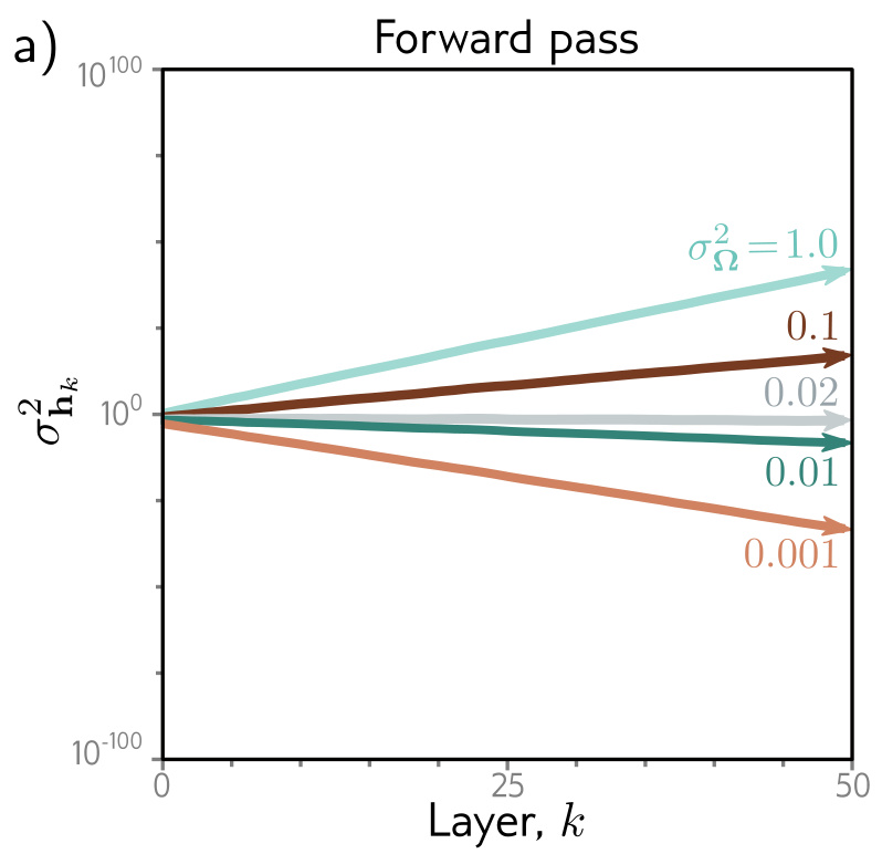
Backpropagation computes the derivatives that SGD and Adam consume; the parameters those algorithms start from still have to be chosen. Consider one pre-activation in the forward pass, \(f_k = \beta_k + \Omega_k a[f_{k-1}]\), with all biases initialized to zero and the elements of \(\Omega_k\) drawn from a normal distribution with mean zero and variance \(\sigma^2\).
- If \(\sigma^2\) is very small — say \(10^{-5}\) — each element of \(\beta_k + \Omega_k h_k\) is a weighted sum of \(h_k\) with very small weights, and so will likely have a smaller magnitude than the input. The ReLU additionally clips values below zero, so the range of \(h_k\) is half that of \(f_{k-1}\). The magnitudes of the pre-activations get smaller and smaller with depth.
- If \(\sigma^2\) is very large — say \(10^5\) — each element is a weighted sum with very large weights and is likely to have a much larger magnitude than the input. The ReLU halves the range, but if \(\sigma^2\) is large enough the magnitudes still grow with depth.
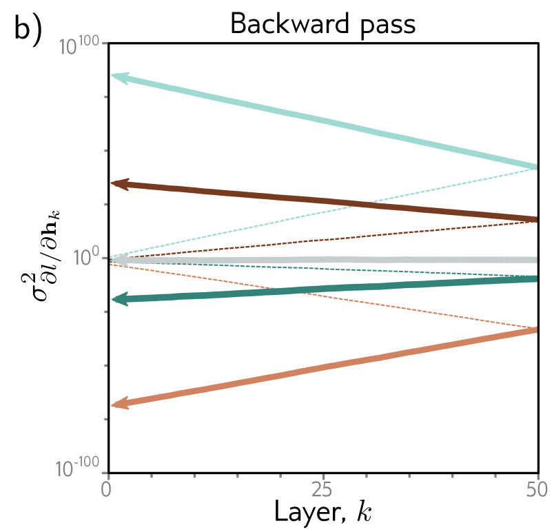
In both situations the pre-activations can become too small or too large to represent in finite-precision floating-point arithmetic. The same logic applies to the backward pass, where each update multiplies by \(\Omega^T\): if the values of \(\Omega\) are not initialized sensibly, gradient magnitudes may decrease or increase uncontrollably. These are the vanishing gradient problem and the exploding gradient problem respectively. In the former, updates become vanishingly small; in the latter, unstable.
The variance argument
Consider adjacent pre-activations \(f\) and \(f'\) with dimensions \(D_h\) and \(D_{h'}\), related by \(h = a[f]\) and \(f' = \beta + \Omega h\), with the pre-activations \(f_j\) in the input layer having variance \(\sigma_f^2\). With biases initialized to zero and weights normally distributed with mean zero and variance \(\sigma_\Omega^2\), the expectation of \(f'_i\) is
\[\mathbb{E}[f'_i] = \mathbb{E}\left[\beta_i + \sum_{j=1}^{D_h}\Omega_{ij}h_j\right] = \mathbb{E}[\beta_i] + \sum_{j=1}^{D_h}\mathbb{E}[\Omega_{ij}]\,\mathbb{E}[h_j] = 0,\]
using the independence of the distributions over the hidden units and the weights. The variance then follows from \(\sigma^2 = \mathbb{E}[z^2] - \mathbb{E}[z]^2\):
\[\sigma_{f'}^2 = \mathbb{E}\left[\left(\sum_{j=1}^{D_h}\Omega_{ij}h_j\right)^2\right] = \sum_{j=1}^{D_h}\mathbb{E}[\Omega_{ij}^2]\,\mathbb{E}[h_j^2] = \sigma_\Omega^2\sum_{j=1}^{D_h}\mathbb{E}[h_j^2].\]
The remaining step is where the factor of two comes from. Assuming the distribution of pre-activations \(f_j\) at the previous layer is symmetric about zero, half of them are clipped by the ReLU function, and the second moment \(\mathbb{E}[h_j^2]\) is half the variance \(\sigma_f^2\) of \(f_j\):
\[\sigma_{f'}^2 = \sigma_\Omega^2\sum_{j=1}^{D_h}\frac{\sigma_f^2}{2} = \frac{1}{2}D_h\sigma_\Omega^2\sigma_f^2.\]
Requiring \(\sigma_{f'}^2 = \sigma_f^2\), so that the variance is unchanged from layer to layer, gives
\[\sigma_\Omega^2 = \frac{2}{D_h},\]
where \(D_h\) is the dimension of the original layer to which the weights were applied. This is He initialization. A similar argument for the backward pass, where gradients are multiplied by the transpose \(\Omega^T\), gives \(\sigma_\Omega^2 = 2/D_{h'}\), where \(D_{h'}\) is the dimension of the layer the weights feed into. When \(\Omega\) is not square the two conditions cannot be satisfied simultaneously, and one compromise uses the mean \((D_h + D_{h'})/2\) as a proxy for the number of terms, giving \(\sigma_\Omega^2 = 4/(D_h + D_{h'})\).
The training loop
The pieces assemble into a short script. The following code, from figure 7.8 of the chapter, defines a two-layer network, initializes the weights, and trains it with SGD with momentum and a decaying learning rate.
import torch, torch.nn as nn
from torch.utils.data import TensorDataset, DataLoader
from torch.optim.lr_scheduler import StepLR

# define input size, hidden layer size, output size
D_i, D_k, D_o = 10, 40, 5
# create model with two hidden layers
model = nn.Sequential(
    nn.Linear(D_i, D_k),
    nn.ReLU(),
    nn.Linear(D_k, D_k),
    nn.ReLU(),
    nn.Linear(D_k, D_o))

# He initialization of weights
def weights_init(layer_in):
    if isinstance(layer_in, nn.Linear):
        nn.init.kaiming_normal_(layer_in.weight)
        layer_in.bias.data.fill_(0.0)
model.apply(weights_init)

# choose least squares loss function
criterion = nn.MSELoss()
# construct SGD optimizer and initialize learning rate and momentum
optimizer = torch.optim.SGD(model.parameters(), lr = 0.1, momentum=0.9)
# object that decreases learning rate by half every 10 epochs
scheduler = StepLR(optimizer, step_size=10, gamma=0.5)

# create 100 random data points and store in data loader class
x = torch.randn(100, D_i)
y = torch.randn(100, D_o)
data_loader = DataLoader(TensorDataset(x,y), batch_size=10, shuffle=True)

# loop over the dataset 100 times
for epoch in range(100):
    epoch_loss = 0.0
    # loop over batches
    for i, data in enumerate(data_loader):
        # retrieve inputs and labels for this batch
        x_batch, y_batch = data
        # zero the parameter gradients
        optimizer.zero_grad()
        # forward pass
        pred = model(x_batch)
        loss = criterion(pred, y_batch)
        # backward pass
        loss.backward()
        # SGD update
        optimizer.step()
        # update statistics
        epoch_loss += loss.item()
    # print error
    print(f'Epoch {epoch:5d}, loss {epoch_loss:.3f}')
    # tell scheduler to consider updating learning rate
    scheduler.step()
All of the details of backpropagation are hidden in the single line loss.backward().
Learning outcomes
- initialize-parameters Initialize weights so activations and gradients neither vanish nor explode.
- compute-gradients-by-backprop Compute the gradients of a deep network’s loss by backpropagation.
Concepts
- he-initialization weights drawn from a zero-mean normal with variance \(2/D_h\) and zero biases hold the activation variance constant across ReLU layers, and \(4/(D_h+D_{h'})\) compromises between the forward and backward conditions
- vanishing-exploding-gradients weight variance away from the prescribed value makes activation and gradient magnitudes change exponentially with depth
- forward-pass the condition \(\sigma_{f'}^2 = \sigma_f^2\) is what keeps the pre-activation variance constant as data moves forward
- backward-pass multiplication by \(\Omega^T\) makes the receiving layer’s dimension \(D_{h'}\) the relevant one for gradient stability
Sources of test error
A trained model is judged on data it was not fitted to. The MNIST-1D dataset makes the gap visible: ten classes \(y \in \{0,1,\dots,9\}\) representing the digits, each example created by randomly transforming one of ten 1D templates and adding noise, giving \(I = 4000\) training examples of \(D_i = 40\) dimensions with roughly 400 examples of each class. A network with \(D_i = 40\) inputs, two hidden layers of \(D = 100\) units, and \(D_o = 10\) outputs passed through a softmax was trained with SGD, batch size 100 and learning rate 0.1 for 6000 steps with the multiclass cross-entropy loss. The training data are classified perfectly after about 4000 steps and the training loss approaches zero.
Perfect training performance does not imply a perfect classifier; the model might have memorised the training set. Evaluated on 1000 further examples generated by the same process, the test errors decrease during training but only to around 40% — better than the chance error rate of 90%, but far worse than on the training set. The test loss behaves differently again: it decreases for the first 1500 training steps and then increases, because the error rate is by then roughly constant while confidence keeps rising. The model makes the same mistakes with increasing certainty, and the negative log-likelihood grows. That rise is a side-effect of the softmax, whose pre-softmax activations are driven to increasingly extreme values to push the probability of the training data towards one.
To make the sources of the gap visible, the chapter reverts to a 1D least squares regression problem in which the data generation is known exactly: a quasi-sinusoidal function, with training and test data produced by sampling inputs in \([0,1]\), passing them through the function, and adding Gaussian noise of fixed variance. The model is a simplified shallow network whose input-to-hidden weights and biases are fixed so that the joints of the function are evenly spaced at \(0, 1/D, 2/D, \dots, (D-1)/D\) for \(D\) hidden units. It can represent any piecewise linear function with \(D\) equally sized regions on \([0,1]\), and it can be fit in closed form, which removes the variability of stochastic optimization and guarantees that the global minimum is found.
Three sources of error are then separable.
Noise. The data generation process adds noise, so there are multiple possible valid outputs \(y\) for each input \(x\). This source of error is insurmountable for the test data. It does not necessarily limit training performance, since the same input \(x\) will likely never be seen twice during training.
Noise may arise from a genuinely stochastic element in the data generation process, from mislabelled data, or from further explanatory variables that were not observed.
Bias. The model may not be flexible enough to fit the true function perfectly. The three-region network cannot exactly describe the quasi-sinusoidal function even when its parameters are chosen optimally.
Variance. The training examples are limited, and there is no way to distinguish systematic changes in the underlying function from noise in the data. For different training datasets the fitted function differs each time, and this variability in the fit is a further source of error. In practice there may be additional variance from the stochastic learning algorithm, which does not necessarily converge to the same solution each time.
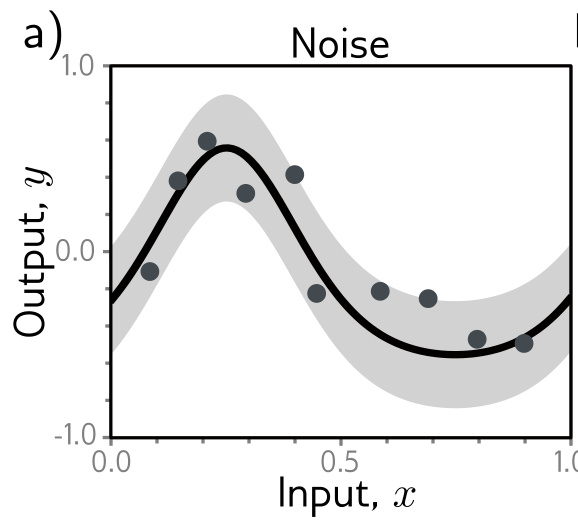
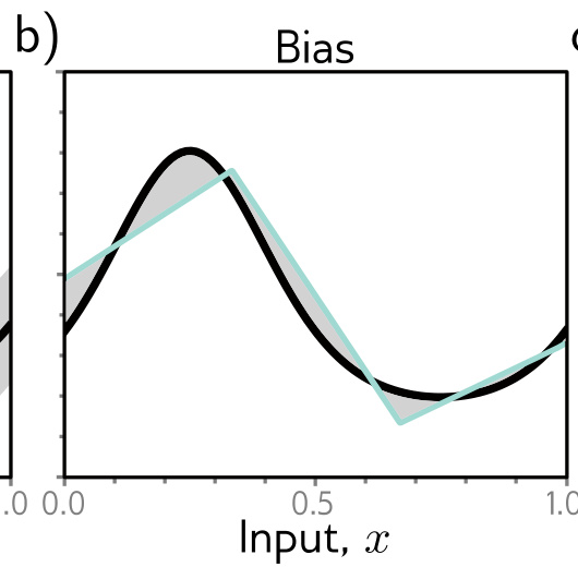
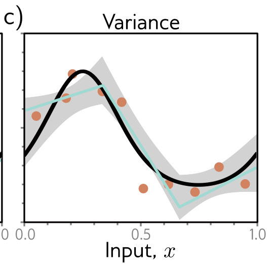
The decomposition
For each input \(x\) there is a distribution \(Pr(y|x)\) with mean \(\mu[x] = \mathbb{E}_y[y[x]] = \int y[x]Pr(y|x)dy\) and fixed noise \(\sigma^2 = \mathbb{E}_y[(\mu[x]-y[x])^2]\). Adding and subtracting \(\mu[x]\) inside the least squares loss \(L[x] = (f[x,\phi]-y[x])^2\) and taking the expectation over \(y\) gives
\[\mathbb{E}_y\big[L[x]\big] = \big(f[x,\phi]-\mu[x]\big)^2 + \sigma^2,\]
because the cross term contains \(\mu[x] - \mathbb{E}_y[y[x]]\), which is zero by definition. The parameters depend on the training dataset \(\mathcal{D}\), so writing \(f[x,\phi[\mathcal{D}]]\) and defining the expected model output \(f_\mu[x] = \mathbb{E}_\mathcal{D}\big[f[x,\phi[\mathcal{D}]]\big]\), the same manoeuvre applied to the first term yields
\[\mathbb{E}_\mathcal{D}\Big[\mathbb{E}_y\big[L[x]\big]\Big] = \underbrace{\mathbb{E}_\mathcal{D}\Big[\big(f[x,\phi[\mathcal{D}]]-f_\mu[x]\big)^2\Big]}_{\text{variance}} + \underbrace{\big(f_\mu[x]-\mu[x]\big)^2}_{\text{bias}} + \underbrace{\sigma^2}_{\text{noise}}.\]
The variance is uncertainty in the fitted model due to the particular training sample; the bias is the systematic deviation of the model from the mean of the function being modelled; the noise is the inherent uncertainty in the true mapping. These three combine additively for regression tasks with a least squares loss, though their interaction can be more complex for other types of problem.
What to change
The noise component is insurmountable and represents a fundamental limit on expected performance. The other two admit remedies.
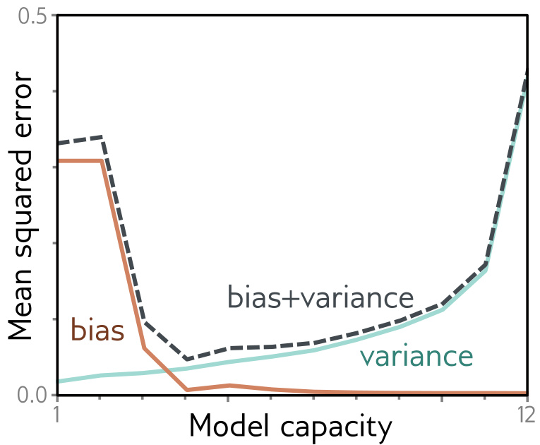
- Variance results from limited noisy training data, so it is reduced by increasing the quantity of training data, which averages out the inherent noise and ensures the input space is well sampled. Fitting the toy model to datasets of 6, 10 and 100 samples shows the fitted functions becoming very similar and the variance shrinking as the sample grows.
- Bias results from the model’s inability to describe the true function, so it is reduced by making the model more flexible — increasing the capacity by adding hidden units or hidden layers. Increasing the toy model from three to ten linear regions makes it flexible enough to fit the true function closely.
Increasing capacity has an unwanted side-effect. For a fixed-size training dataset the variance term typically increases as capacity increases, so increasing capacity does not necessarily reduce the test error. This is the bias-variance trade-off. Fitting the three-region model to three different datasets of fifteen points produces nearly the same result each time, since the noise roughly averages out in each linear region; fitting a ten-region model to the same three datasets fits the data better, but much of the extra descriptive power is devoted to modelling the noise, which is overfitting. For regression the total expected error is the sum of the bias and the variance, and for the toy model on fifteen points that sum is minimized when the capacity is four.
Learning outcomes
- decompose-test-error Decompose test error into noise, bias, and variance, and diagnose which dominates.
Concepts
- generalization performance is judged on a separate test set, and zero training error on MNIST-1D coexists with roughly 40% test error
- noise-bias-variance-decomposition the expected least squares test error is the sum of a variance term, a squared bias term and the irreducible noise variance
- bias-variance-trade-off for a fixed dataset size, capacity that lowers bias raises variance, so the sum is minimized at an intermediate capacity
Double descent and model selection
Returning to MNIST-1D with 10,000 training examples, 5,000 further test examples, and a model trained with Adam at a step size of 0.005 on a full batch of 10,000 examples for 4000 steps, the classical picture does not appear. As the number of hidden units in each of two layers grows, the training error decreases to near zero, and the vertical line marking the capacity at which the model has as many parameters as there are training examples is passed well after the dataset has been memorised. The test error decreases as capacity is added and does not increase as the bias-variance trade-off predicts; it keeps decreasing.
Repeating the experiment with 15% of the training labels randomized makes both phenomena visible at once. The training error again decreases to zero, though now almost as many parameters as data points are required to memorise the data. The test error shows the expected trade-off up to the point where the training data are fitted exactly, then does something unexpected: it starts to decrease again, and with enough capacity falls below the minimum achieved in the first part of the curve.
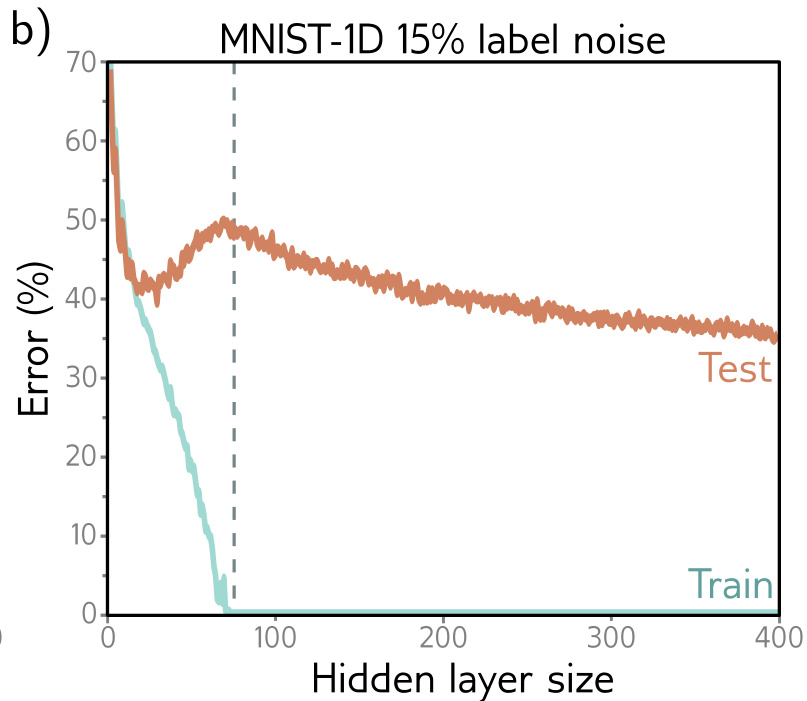
This is double descent. The first part of the curve is the classical or under-parameterized regime, the second the modern or over-parameterized regime, and the central part where the error increases is the critical regime. It is present with the original data for some datasets such as MNIST, and for others, including MNIST-1D and CIFAR-100, it emerges or becomes more prominent when noise is added to the labels.
Why the second descent
The first phenomenon, worsening test performance where the model has just enough capacity to memorise the data, is exactly what the bias-variance trade-off predicts. The second is more confusing: it is unclear why performance should be better in the over-parameterized regime, where there are not even enough training data points to constrain the model parameters uniquely.
Once the model has enough capacity to drive the training loss to near zero it fits the training data almost perfectly, so further capacity cannot help it there; any change must occur between the training points. The tendency of a model to prioritize one solution over another between data points is its inductive bias.
That behaviour matters because in high-dimensional space the training data are extremely sparse. MNIST-1D has 40 dimensions and the experiment used 10,000 examples. Quantizing each input dimension into 10 bins gives \(10^{40}\) bins in total, constrained by only \(10^4\) examples — even with this coarse quantization there is only one data point in every \(10^{36}\) bins. The tendency of the volume of high-dimensional space to overwhelm the number of training points is the curse of dimensionality.
The putative explanation is that as capacity is added the model interpolates between the nearest data points increasingly smoothly. In the absence of information about what happens between the training points, assuming smoothness is sensible and will probably generalize reasonably to new data. Plotting the smoothest possible functions that still pass through a sparse set of points as the number of hidden units rises from 6 to 50 supports the first half of the claim: when the parameter count is very close to the number of training examples the model is forced to contort itself to fit the data exactly, producing erratic predictions, which explains why the peak is so pronounced; with more hidden units it has the ability to construct smoother functions.
The argument is incomplete. Having the ability to produce a smooth function does not oblige a model to do so — three quite different functions produced by the simplified model with 50 hidden units all fit the data exactly, so the loss is zero for each. Any factor that biases a model towards a subset of the solutions with a similar training loss is a regularizer. Two possibilities are that the initialization encourages smoothness and the model never departs from the sub-domain of smooth functions during training, or that the training algorithm itself acts as an implicit regularizer.
Choosing hyperparameters
In the classical regime neither the bias nor the variance is accessible: the bias requires knowledge of the true underlying function and the variance requires multiple independently sampled datasets. In the modern regime there is no way to tell how much capacity should be added before the test error stops improving. Capacity must therefore be chosen empirically, and so must the number of hidden layers, other aspects of architecture, and the learning algorithm and its parameters — collectively the hyperparameters. Finding the best ones is hyperparameter search, or neural architecture search when focused on network structure.
Training many models on the same training set and retaining the one that performs best on the test set would admit the possibility that these hyperparameters happen to work well for that test set but do not generalize further. A third dataset is introduced instead, the validation set. For every choice of hyperparameters the associated model is trained on the training set and evaluated on the validation set; the model that worked best on the validation set is selected, and its performance is measured on the test set.
The search is not a gradient problem. The hyperparameter space is smaller than the parameter space but still too large to try every combination exhaustively; many hyperparameters are discrete, such as the number of hidden layers; and others are conditional on one another, so that the number of hidden units in the tenth hidden layer need only be specified if there are ten or more layers. Hyperparameter optimization algorithms therefore sample the space intelligently, contingent on previous results. One approach is to sample the space randomly. For continuous variables it is better to build a model of performance as a function of the hyperparameters together with the uncertainty in that function, which can be exploited to test where the uncertainty is great or to home in on promising regions; Bayesian optimization is a framework based on Gaussian processes that does this. The procedure is expensive, since an entire model must be trained and its validation performance measured for each combination.
A good test score is still not a guarantee. If the statistics of the test set do not match those of real-world data, or change over time, deployed performance will be worse — dataset shift. The input statistics of \(x\) may change, so that parts of the function sparsely sampled or unsampled during training are now being observed, which is covariate shift; the statistics of the output \(y\) may change, so that values infrequent during training are more common in the real world, which is prior shift; or the relationship between input and output may change, which is concept shift.
Learning outcomes
- explain-double-descent Explain double descent and why over-parameterized networks defy the classical bias-variance curve.
- select-hyperparameters Use a validation split to select hyperparameters without contaminating the test set.
- decompose-test-error Decompose test error into noise, bias, and variance, and diagnose which dominates.
Concepts
- double-descent test error peaks at the capacity where the training data are exactly memorized and then falls again through the over-parameterized regime
- bias-variance-trade-off the classical curve accounts for the first ascent but not for the second descent that deep networks exhibit
- curse-of-dimensionality with \(10^{40}\) quantization bins constrained by \(10^4\) examples, what the model does between training points determines its test error
- implicit-regularization many functions attain zero training loss, so something in the initialization or the optimizer must be selecting the smooth ones
- hyperparameter-optimization hyperparameters are selected on a validation set and the test set is reserved for the final estimate, because the space is discrete, conditional and non-differentiable
- generalization tuning on the test set would report a score that need not hold for further data
- dataset-shift deployed performance can fall below the test score through covariate, prior or concept shift
Explicit and implicit regularization
Regularization is a family of methods that reduce the generalization gap between training and test performance. Strictly it means adding explicit terms to the loss function that favour certain parameter choices, though the term is commonly used for any strategy that improves generalization.
In its strict sense, an additional term is included in the objective:
\[\hat{\phi} = \underset{\phi}{\operatorname{argmin}}\left[\sum_{i=1}^{I}\ell_i[x_i,y_i] + \lambda\cdot g[\phi]\right],\]
where \(g[\phi]\) returns a scalar taking larger values when the parameters are less preferred, and the positive scalar \(\lambda\) controls the relative contribution of the two terms. The minima of the regularized loss usually differ from those of the original, so training converges to different parameter values. On the Gabor model loss surface the effect is visible: adding a penalty that grows away from the centre of the plot leaves a surface with fewer local minima and a global minimum in a different position.
The probabilistic reading
Section 5.1 constructed losses from the maximum likelihood criterion \(\hat{\phi} = \operatorname{argmax}_\phi[\prod_{i=1}^I Pr(y_i|x_i,\phi)]\). The regularization term can be considered a prior \(Pr(\phi)\) representing knowledge about the parameters before the data are observed, which gives the maximum a posteriori or MAP criterion
\[\hat{\phi} = \underset{\phi}{\operatorname{argmax}}\left[\prod_{i=1}^{I}Pr(y_i|x_i,\phi)Pr(\phi)\right].\]
Taking the log and multiplying by minus one to return to the negative log-likelihood loss shows that \(\lambda\cdot g[\phi] = -\log[Pr(\phi)]\). The penalty is the negative log of a prior.
L2 regularization
Which solutions the term should penalize is a separate question, and because neural networks are used across an extremely broad range of applications the preferences can only be very generic. The most commonly used regularization term is the L2 norm, which penalizes the sum of the squares of the parameter values:
\[\hat{\phi} = \underset{\phi}{\operatorname{argmin}}\left[\sum_{i=1}^{I}\ell_i[x_i,y_i] + \lambda\sum_j \phi_j^2\right].\]
This is also referred to as Tikhonov regularization or ridge regression, or, applied to matrices, Frobenius norm regularization. For neural networks it is usually applied to the weights but not the biases and is then called a weight decay term.
The mechanism is smoothing. The output prediction is a weighted sum of the activations at the last hidden layer, so if the weights have a smaller magnitude the output will vary less. The same logic applies to the computation of the pre-activations at the last hidden layer and so on, progressing backward through the network. In the limit, forcing all the weights to zero would make the network produce a constant output determined by the final bias parameter.
Fitting the simplified network with 14 hidden units under increasing \(\lambda\) shows the consequence. For small \(\lambda\) — \(0\) and \(0.00001\) — the fitted function passes exactly through the data points. For intermediate \(\lambda\) — \(0.0001\) and \(0.001\) — it is smoother and more similar to the ground truth. For large \(\lambda\) — \(0.01\) and \(0.1\) — the regularization term overpowers the likelihood term, the function is too smooth, and the overall fit is worse. Test performance may improve for two reasons: if the network is overfitting, the term forces a trade-off between slavish adherence to the data and smoothness, reducing the error due to variance at the cost of increased bias; and if the network is over-parameterized, some of the extra capacity describes areas with no training data, where the term favours functions that interpolate smoothly between the nearby points.
The optimizer regularizes on its own
Neither gradient descent nor stochastic gradient descent moves neutrally to the minimum of the loss function; each exhibits a preference for some solutions over others. This is implicit regularization.
Consider a continuous version of gradient descent in which the step size is infinitesimal, so that the parameters are governed by the differential equation \(d\phi/dt = -\partial L/\partial\phi\). Gradient descent approximates this process with a series of discrete steps of size \(\alpha\), and the discretization causes a deviation from the continuous path. A modified loss \(\tilde{L}\) can be derived whose continuous trajectory arrives where the discretized version on the original loss \(L\) does, and by backward error analysis it is
\[\tilde{L}_{GD}[\phi] = L[\phi] + \frac{\alpha}{4}\left\|\frac{\partial L}{\partial\phi}\right\|^2.\]
The discrete trajectory is repelled from places where the gradient norm is large — that is, where the surface is steep. This does not change the position of the minima, where the gradients are zero anyway, but it changes the effective loss function elsewhere and modifies the trajectory, which may converge to a different minimum. It may be responsible for the observation that full batch gradient descent generalizes better with larger step sizes.
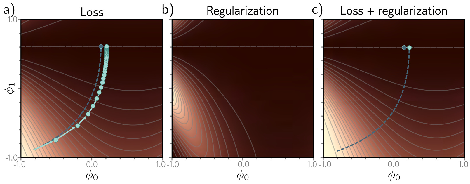
The same analysis applied to SGD — seeking a modified loss whose continuous version reaches the same place as the average of the possible random SGD updates — gives
\[\tilde{L}_{SGD}[\phi] = L[\phi] + \frac{\alpha}{4}\left\|\frac{\partial L}{\partial\phi}\right\|^2 + \frac{\alpha}{4B}\sum_{b=1}^{B}\left\|\frac{\partial L_b}{\partial\phi}-\frac{\partial L}{\partial\phi}\right\|^2,\]
where \(L_b\) is the loss for the \(b^{th}\) of the \(B\) batches in an epoch, and \(L\) and \(L_b\) are now the means of the \(I\) individual losses in the full dataset and of the \(|\mathcal{B}|\) individual losses in the batch respectively. The extra term is the variance of the gradients of the batch losses: SGD implicitly favours places where the batch gradients agree. If the model is over-parameterized and fits all the training data exactly, each of these gradient terms is zero at the global minimum, so the position of that minimum need not move; the trajectory does.
Empirically SGD generalizes better than gradient descent, and smaller batch sizes generally perform better than larger ones. One possible explanation is that the inherent randomness allows the algorithm to reach different parts of the loss function. It is also possible that some or all of the performance increase is due to implicit regularization, which encourages solutions where all the data fits well — so that the batch variance is small — rather than solutions where some data fits extremely well and other data less well, perhaps with the same overall loss but larger batch variance. The former are likely to generalize better.
Learning outcomes
- apply-explicit-regularization Add an explicit regularization term and read it as a prior over parameters.
- recognize-implicit-regularization Recognize that gradient descent and SGD regularize on their own.
Concepts
- explicit-regularization adding \(\lambda\cdot g[\phi]\) to the loss moves the minima, and the term is the negative log of a prior over the parameters, making the result a MAP estimate
- bayesian-inference the prior \(Pr(\phi)\) that the penalty encodes is the same prior that appears in the numerator of Bayes’ rule
- l2-regularization penalising \(\sum_j \phi_j^2\) drives the weights smaller, and smaller weights make the output function vary less
- implicit-regularization the finite step size adds a penalty \(\frac{\alpha}{4}\|\partial L/\partial\phi\|^2\) on the gradient norm, and minibatch sampling adds a further penalty on the variance between batch gradients
Regularization heuristics
Beyond the explicit term and the optimizer’s own preferences, a set of practical methods improves generalization. Each works for a reason, and the reason says when it will not.
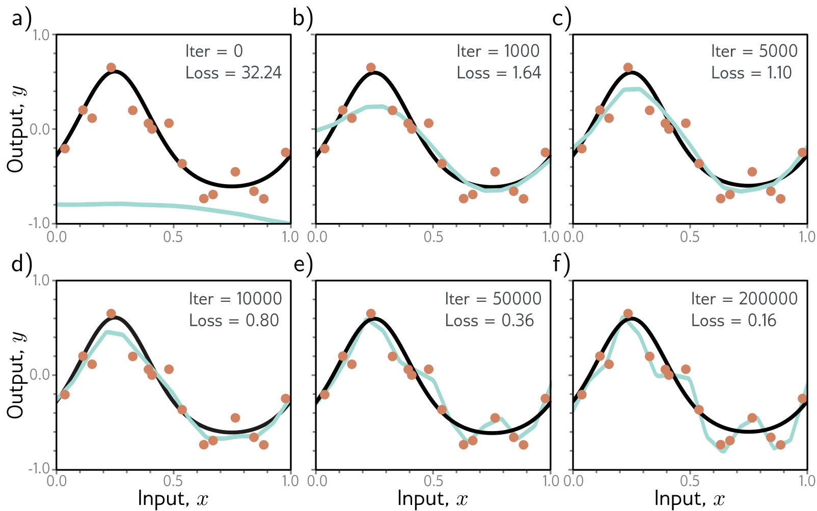
Early stopping stops the training procedure before it has fully converged.
This reduces overfitting if the model has already captured the coarse shape of the underlying function but has not yet had time to overfit to the noise. Since the weights are initialized to small values, they simply do not have time to become large, so early stopping has a similar effect to explicit L2 regularization. A different view is that it reduces the effective model complexity, moving back down the bias-variance trade-off curve from the critical region.
Its single hyperparameter is the number of steps after which learning is terminated, and it is chosen without training multiple models: the model is trained once, performance on the validation set is monitored every \(T\) iterations, and the parameters where validation performance was best are selected.
Ensembling builds several models and averages their predictions.
The models are combined by taking the mean of the outputs for regression problems or the mean of the pre-softmax activations for classification, on the assumption that model errors are independent and will cancel out. Alternatively the median of the outputs or the most frequent predicted class makes the predictions more robust. One way to train different models is to use different random initializations, which may help in regions of input space far from the training data, where the fitted function is relatively unconstrained.
Bootstrap aggregating, or bagging, generates several different datasets by re-sampling the training data with replacement and trains a different model from each.
It has the effect of smoothing out the data: if a point is not present in one training set the model interpolates from nearby points, so if that point was an outlier the fitted function is more moderate in that region.
Dropout clamps a random subset of hidden units, typically 50%, to zero at each iteration of SGD.
This makes the network less dependent on any given hidden unit and encourages the weights to have smaller magnitudes, so the change in the function due to the presence or absence of any specific unit is reduced. It also eliminates undesirable kinks in the function that are far from the training data and do not affect the loss. Three hidden units becoming active in sequence can conspire to raise, lower, and restore the slope, producing a local change that will not change the training loss but is unlikely to generalize well. Removing one of them, as dropout does, causes a considerable change to the output in the half-space where that unit was active; the subsequent gradient descent step compensates, and such dependencies are eliminated over time.
At test time the network can be run as usual with all the hidden units active, but it now has more hidden units than it was trained with at any given iteration, so the weights are multiplied by one minus the dropout probability to compensate. This is the weight scaling inference rule. Monte Carlo dropout instead runs the network multiple times with different random subsets clamped to zero and combines the results, which is closely related to ensembling — every random version of the network is a different model — without training or storing multiple networks.
Applying noise generalizes dropout, which can be interpreted as applying multiplicative Bernoulli noise to the activations.
Adding noise to the inputs smooths out the learned function; for regression problems it can be shown to be equivalent to adding a regularizing term that penalizes the derivatives of the network’s output with respect to its input. Adversarial training is an extreme variant in which the optimization algorithm actively searches for small perturbations of the input that cause large changes in the output. Adding noise to the weights encourages the network to make sensible predictions under small perturbations of the weights, so training converges to local minima in the middle of wide, flat regions.
Label smoothing perturbs the targets instead.
The maximum-likelihood criterion for multiclass classification aims to predict the correct class with absolute certainty, which drives the pre-softmax activations to very large values for the correct class and very small ones for the wrong classes. Assuming that a proportion \(\rho\) of the training labels are incorrect and belong with equal probability to the other classes discourages this: the loss is changed to minimize the cross-entropy between the predicted distribution and a distribution where the true label has probability \(1-\rho\) and the other classes have equal probability.
Bayesian inference is the principled limit of treating the parameters as uncertain.
The parameters are given a distribution \(Pr(\phi|\{x_i,y_i\})\) conditioned on the training data through Bayes’ rule, and the prediction for a new input is \(Pr(y|x,\{x_i,y_i\}) = \int Pr(y|x,\phi)Pr(\phi|\{x_i,y_i\})d\phi\). This is effectively an infinite weighted ensemble, where the weight depends on the prior probability of the parameters and on their agreement with the data. For complex models like neural networks there is no practical way to represent the full distribution over the parameters or to integrate over it, so all current methods of this type make approximations and typically add considerable complexity.
Transfer learning exploits a different dataset when training data for the task at hand are limited.
The network is pre-trained to perform a related secondary task for which data are more plentiful. The resulting model is adapted to the original task, typically by removing the last layer and adding one or more layers that produce a suitable output; the main model may be fixed and only the new layers trained, or the entire model may be fine-tuned. The principle is that the network builds a good internal representation of the data from the secondary task, which can then be exploited. Equivalently, transfer learning initializes most of the parameters in a sensible part of the space.
Multi-task learning trains the network to solve several problems concurrently.
A network might take an image and simultaneously learn to segment the scene, estimate the pixel-wise depth, and predict a caption. All of these tasks require some understanding of the image, and learned simultaneously the performance on each may improve.
Self-supervised learning manufactures the secondary task from unlabelled data.
In generative self-supervised learning part of each data example is masked and the secondary task is to predict the missing part — inpainting missing parts of images from a corpus of unlabelled images, or predicting masked words in a corpus of text. In contrastive self-supervised learning pairs of examples with commonalities are compared to unrelated pairs, so the task might be to identify whether a pair of images are transformed versions of one another or whether two sentences followed one another in the original document.
Data augmentation expands the dataset instead of borrowing another one.
Each input example is transformed in a way that leaves the label unchanged: an image can be rotated, flipped, blurred or have its colour balance manipulated, and the label “bird” remains valid. Where the input is text, synonyms can be substituted or the text translated to another language and back; where it is audio, different frequency bands can be amplified or attenuated. The aim is to teach the model to be indifferent to these irrelevant data transformations.
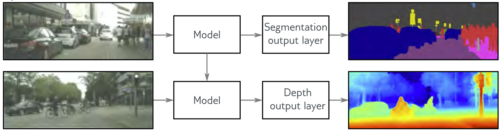
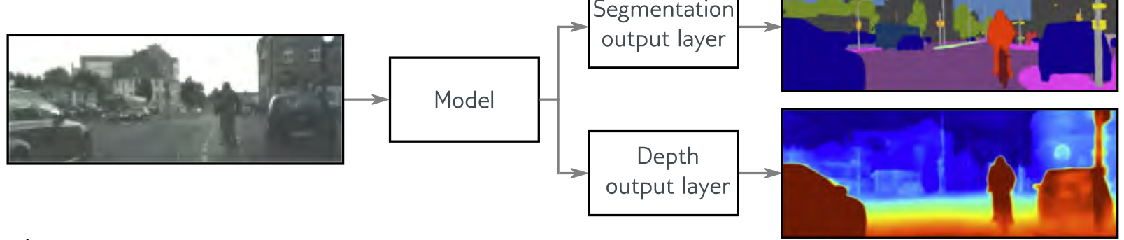

The chapter’s summary organises all of these by mechanism. There are four: make the modelled function smoother, as L2 regularization, early stopping and input noise do; increase the effective amount of data, as augmentation, transfer learning and multi-task learning do; combine multiple models, as ensembling, the Bayesian approach and dropout do; and find wider minima, where small errors in the estimated parameters matter less, as implicit regularization and noise on the weights do.
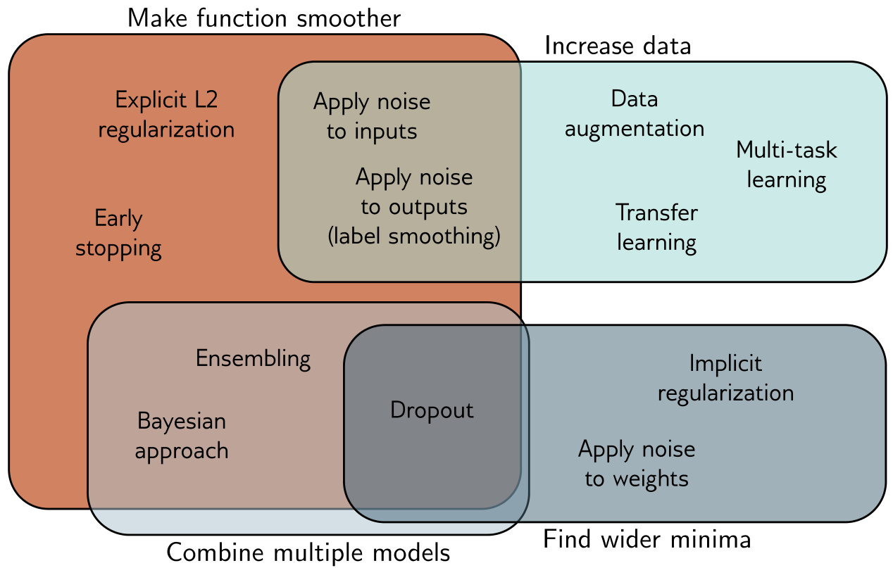
Learning outcomes
- apply-regularization-heuristics Apply practical regularizers — early stopping, dropout, ensembling, augmentation, transfer learning.
- decompose-test-error Decompose test error into noise, bias, and variance, and diagnose which dominates.
Concepts
- early-stopping halting at the best validation performance leaves the weights near their small initial values, which limits the effective complexity of the model
- l2-regularization early stopping has a similar effect to the explicit weight penalty, because the weights do not have time to grow large
- ensembling averaging several models trained from different initializations or on bootstrap resamples cancels errors that are independent between them
- dropout clamping a random half of the hidden units to zero at each iteration removes co-adaptations and kinks that do not affect the training loss
- noise-injection noise on the inputs smooths the learned function, noise on the weights favours wide minima, and label smoothing replaces a one-hot target with \(1-\rho\) on the true class
- bayesian-inference predicting by an integral weighted by the parameter posterior is an infinite ensemble, and is approximated in practice
- transfer-and-multitask-learning pre-training on a data-rich secondary task, or learning several tasks at once, supplies a representation that a scarce-label task can reuse
- self-supervised-learning masking part of an example or contrasting related pairs manufactures labels from unlabelled data
- data-augmentation label-preserving transformations of each example enlarge the dataset and teach indifference to those transformations
Conclusion
Neural networks compute the parameters of conditional probability distributions over the targets rather than the targets themselves.
That single change of perspective supplies a recipe: choose a distribution over the output domain, predict its parameters, minimize negative log-likelihood, and read off inference from the fitted distribution.
Least squares, binary cross-entropy and multiclass cross-entropy are algebraic reductions of one criterion under three distributional choices.
Nothing is chosen by convention. A normal output gives sum of squares, a Bernoulli output with a sigmoid gives binary cross-entropy, and a categorical output with a softmax gives multiclass cross-entropy.
Minimizing negative log-likelihood is minimizing the KL divergence from the empirical data distribution to the model distribution.
Cross-entropy and maximum likelihood are two names for the same objective, so a claim proved for one holds for the other.
The success of the update rule depends on the geometry of the loss surface, not on the rule.
Convex surfaces guarantee that descent reaches the global minimum; the non-convex surfaces of neural networks hold local minima and saddle points, which is what SGD, momentum and Adam exist to mitigate.
Backpropagation computes every parameter derivative in two passes by calculating each shared intermediate quantity once.
The forward pass stores the activations because each weight derivative is proportional to the activation at its source; the backward pass exploits the redundancy the reverse order exposes. The cost is memory, not arithmetic.
Weight variance decides whether signals survive depth, and He initialization sets it to \(2/D_h\).
The factor of two accounts for the ReLU halving the second moment of the pre-activations. Departing from this value makes activations and gradients change exponentially in the number of layers.
Test error decomposes additively into noise, bias and variance for regression with a least squares loss.
Which term dominates decides the response: more data reduces variance, more capacity reduces bias, and nothing reduces noise.
Test error can fall again beyond the interpolation threshold, and what the optimizer prefers among the zero-loss solutions is part of the reason.
Gradient descent with a finite step size penalizes the gradient norm and SGD additionally penalizes the variance between batch gradients, so the algorithm is already a regularizer before any term is added to the loss.
Everything so far applies to a fully connected network acting on an unstructured input vector. For an image that is a poor fit: the parameter count explodes with resolution, and the model learns nothing from the fact that neighbouring pixels are related. The next unit, Convnets, replaces the fully connected layer with convolution — a shared kernel that slides across the input, giving weight sharing and translation equivariance — and controls what each unit sees through kernel size, stride, padding and dilation. It also confronts a training difficulty this unit’s tools do not resolve: very deep plain networks reach a higher training loss than shallower ones, an optimization failure rather than a capacity failure, which residual connections and batch normalization address.
References
- Understanding Deep Learning, Simon Prince, 2026 — Link — Pages 70-90, 91-109, 110-131, 132-151, 152-174