Maximum likelihood and the negative log-likelihood
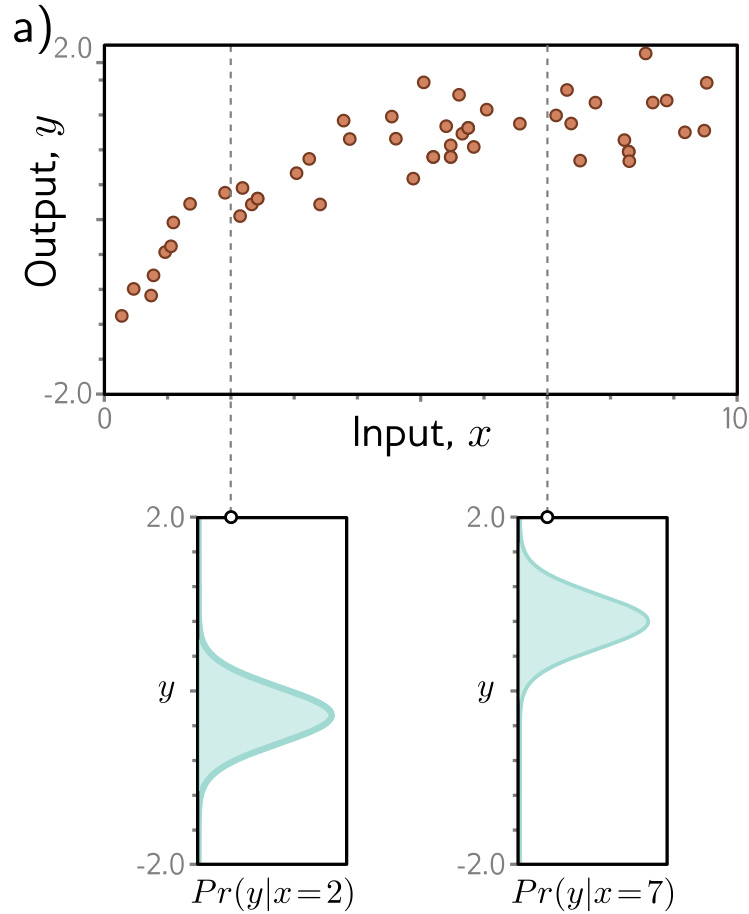
The model predicts a distribution
One distribution per output domain.
Until now \(f[x,\phi]\) returned a value \(y\)
Now it returns a conditional distribution \(Pr(y|x)\)
Real values, classes, counts, directions — each has its own family
Two models, not one
The probability model
\[Pr(y|\theta)\]
Chosen by hand, once, from the output domain. Fixed for the task.
The machine learning model
\[\theta = f[x,\phi]\]
Learned from data. Computes the parameters of the first .
The network never predicts \(y\) . It predicts what governs \(y\) .
Keeping these separate is what makes the rest of the section mechanical. Changing the task changes only the first model; the second is a network either way.
The maximum likelihood criterion
Each input yields its own \(\theta_i = f[x_i,\phi]\) . Maximise the combined probability:
\[\hat{\phi} = \underset{\phi}{\operatorname{argmax}} \left[ \prod_{i=1}^{I} Pr(y_i|f[x_i,\phi]) \right]\]
Two assumptions, together the i.i.d. assumption:
identically distributed — one distributional form everywhereindependent — so the likelihood factorises
From a product to a sum
Take the logarithm
\[\hat{\phi} = \underset{\phi}{\operatorname{argmax}} \left[ \sum_{i=1}^{I} \log\big[Pr(y_i|f[x_i,\phi])\big] \right]\]
A product of \(I\) small factors underflows finite precision.
Then negate
\[L[\phi] = -\sum_{i=1}^{I} \log\big[Pr(y_i|f[x_i,\phi])\big]\]
Fitting is framed as minimisation, so \(\hat{\phi} = \operatorname{argmin}_\phi\big[L[\phi]\big]\) .
The maximiser does not move: the logarithm is strictly monotonically increasing, so if \(z > z'\) then \(\log[z] > \log[z']\) .
The recipe
Choose a distribution \(Pr(y|\theta)\) over the domain of \(y\)
Set the network to predict its parameters, \(\theta = f[x,\phi]\)
Minimise the negative log-likelihood over the training pairs
At test time return the distribution, or the value maximising it
Steps (2)–(4) never vary. Only the distribution in (1) does: normal, Bernoulli, categorical.
Univariate regression: the normal
\[Pr(y|\mu,\sigma^2) = \frac{1}{\sqrt{2\pi\sigma^2}}\exp\left[-\frac{(y-\mu)^2}{2\sigma^2}\right]\]
Defined for \(y \in \mathbb{R}\)
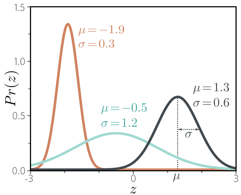
\(\mu\) sets the peak, \(\sigma^2\) the widthStep (2) sets \(\mu = f[x,\phi]\)
Least squares falls out
\[
\begin{aligned}
\hat{\phi} &= \underset{\phi}{\operatorname{argmin}}\left[-\sum_{i=1}^{I}\log\left[\frac{1}{\sqrt{2\pi\sigma^2}}\exp\left[-\frac{(y_i-f[x_i,\phi])^2}{2\sigma^2}\right]\right]\right]\\
&= \underset{\phi}{\operatorname{argmin}}\left[-\sum_{i=1}^{I}\left(\log\left[\frac{1}{\sqrt{2\pi\sigma^2}}\right] - \frac{(y_i-f[x_i,\phi])^2}{2\sigma^2}\right)\right]\\
&= \underset{\phi}{\operatorname{argmin}}\left[\sum_{i=1}^{I}(y_i-f[x_i,\phi])^2\right]
\end{aligned}
\]
The first term drops — no \(\phi\) in it
The \(2\sigma^2\) drops — a constant positive scale
Least squares is a consequence, not a convention.
Heteroscedastic regression
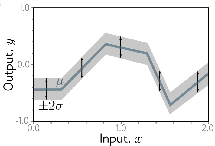
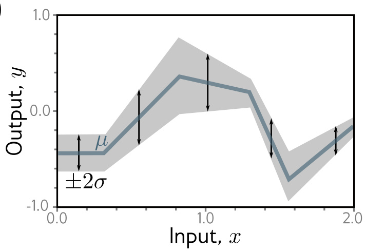
Homoscedastic: constant variance.
Heteroscedastic: variance varies with \(x\) .
A second network output learns the variance: \(\sigma^2 = f_2[x,\phi]^2\) .
The first output predicts the mean, the second the variance. A variance must be positive and a network output need not be, so the second output is squared. Both are learned by the same gradient step on the same loss.
The heteroscedastic loss
\[\hat{\phi} = \underset{\phi}{\operatorname{argmin}}\left[-\sum_{i=1}^{I}\left(\log\left[\frac{1}{\sqrt{2\pi f_2[x_i,\phi]^2}}\right] - \frac{(y_i - f_1[x_i,\phi])^2}{2f_2[x_i,\phi]^2}\right)\right]\]
\(f_1\) predicts the mean, \(f_2^2\) the varianceThe squared error is weighted by the predicted precision
Classification and cross-entropy
Binary classification: the Bernoulli
For \(y \in \{0,1\}\) , one parameter \(\lambda \in [0,1]\) — the probability that \(y = 1\) :
\[Pr(y|\lambda) = (1-\lambda)^{1-y}\cdot\lambda^{y}\]
Step one of the recipe is all that changed
The network must produce a \(\lambda\) inside \([0,1]\)
Predicting whether a restaurant review is positive from its text, or whether a tumour is present in an MRI scan. The value of \(y\) is termed a label.
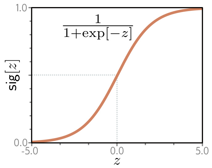
Logit and probability
Zero maps to \(0.5\) .
The network output
\(z = f[x,\phi] \in \mathbb{R}\) — the logit , unconstrained
The distribution parameter
\[\lambda = \operatorname{sig}[z] = \frac{1}{1+\exp[-z]}\]
The sigmoid is what maps an unconstrained output onto a valid parameter.
Binary cross-entropy
Both the label and the model are distributions over the domain \(y \in \{0,1\}\) :
\[\ell_i = -\sum_{y \in \{0,1\}} q_i(y)\,\log\big[p_i(y)\big] = -\,\mathbb{E}_{y\sim q_i}\big[\log p_i(y)\big]\]
The data, \(q_i\)
\(q_i(1) = y_i\) , \(q_i(0) = 1-y_i\)
The model, \(p_i\)
\(p_i(1) = \lambda_i\) , \(p_i(0) = 1-\lambda_i\)
Expanding the two terms: \(-(1-y_i)\log[1-\lambda_i] - y_i\log[\lambda_i]\) .
In terms of the logit
The network emits a logit, so \(\lambda_i = \operatorname{sig}[f[x_i,\phi]]\) . Summing over the training set:
\[L[\phi] = \sum_{i=1}^{I} -(1-y_i)\log\big[1-\operatorname{sig}[f[x_i,\phi]]\big] - y_i \log\big[\operatorname{sig}[f[x_i,\phi]]\big]\]
At inference \(\operatorname{sig}[f[x,\phi]]\) is \(Pr(y=1)\)
A point estimate takes \(y=1\) when \(\lambda > 0.5\)
Multiclass: the categorical distribution
For \(y \in \{1,\dots,K\}\) , \(K\) parameters with \(Pr(y=k) = \lambda_k\) :
each \(\lambda_k \in [0,1]\)
collectively they sum to one
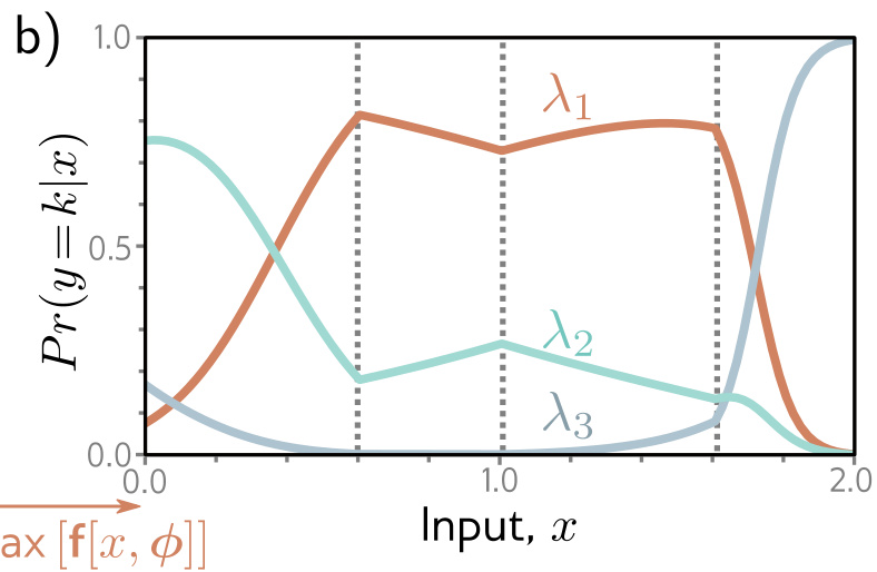
The network produces a logit vector \(z \in \mathbb{R}^K\) , one output per class, with no constraint on any of them.
The softmax
Any vertical slice sums to one.
\[\operatorname{softmax}_k[z] = \frac{\exp[z_k]}{\sum_{k'=1}^{K}\exp[z_{k'}]}\]
the exponentials give positivity
the denominator gives the sum
Multiclass cross-entropy
The same shape, with the domain now \(y \in \{1,\dots,K\}\) :
\[\ell_i = -\sum_{k=1}^{K} q_i(k)\,\log\big[p_i(k)\big] = -\,\mathbb{E}_{y\sim q_i}\big[\log p_i(y)\big]\]
The data, \(q_i\)
\(q_i(k) = \delta[k - y_i]\)
The Kronecker delta: \(1\) at \(k = y_i\) , \(0\) elsewhere.
The model, \(p_i\)
\(p_i(k) = \operatorname{softmax}_k\big[f[x_i,\phi]\big]\)
The delta selects one term, leaving \(\ell_i = -\log p_i(y_i)\) .
The loss in terms of the logits
Substituting the softmax into \(-\log Pr(y_i|\cdot)\) and expanding the logarithm:
\[
\begin{aligned}
L[\phi] &= -\sum_{i=1}^{I}\log\left[\frac{\exp\big[f_{y_i}[x_i,\phi]\big]}{\sum_{k'=1}^{K}\exp\big[f_{k'}[x_i,\phi]\big]}\right]\\
&= -\sum_{i=1}^{I}\left(f_{y_i}[x_i,\phi] - \log\left[\sum_{k'=1}^{K}\exp\big[f_{k'}[x_i,\phi]\big]\right]\right)
\end{aligned}
\]
The correct class’s logit, against the log-sum-exp of all of them.
🎯 Another metric as a loss function: Kullback-Leibler divergence
Training so far minimised a likelihood. The same objective can be posed as a distance between distributions .
The data distribution, \(q\)
fixed by the training set
unknown in closed form, but sampled from
The model distribution, \(p\)
parameterised by \(\theta\)
free to move
Learning becomes: move \(p\) until it is as close as possible to \(q\) .
The Kullback-Leibler divergence is the standard measure of how far one distribution sits from another. It is not symmetric, so it is not a distance in the metric sense, but it is zero exactly when the two distributions agree and positive otherwise – which is all that is needed for it to serve as a loss.
Cross-entropy: the KL divergence
The divergence
\[D_{KL}[q\|p] = \mathbb{E}_{z\sim q}\left[\log\frac{q(z)}{p(z)}\right]\]
Expanding the ratio:
\[
\begin{aligned}
&= \int q(z)\log[q(z)]\,dz\\
&\quad - \int q(z)\log[p(z)]\,dz
\end{aligned}
\]
What depends on \(\theta\)
The first carries no \(\theta\) : it shifts the loss surface by a constant, leaving every gradient unchanged
The second is the cross-entropy — the only term training sees
Substituting the empirical distribution
The data give \(q\) as point masses at the observed outputs:
\[q(y) = \frac{1}{I}\sum_{i=1}^{I}\delta[y-y_i]\]
The cross-entropy term becomes a sum over the training set:
\[-\int q(z)\log[p(z)]\,dz = -\frac{1}{I}\sum_{i=1}^{I}\log\big[Pr(y_i|\theta)\big]\]
The factor \(1/I\) scales the surface, not the location of its minimum.
The same loss the recipe gave
Minimising the divergence
\[-\sum_{i=1}^{I}\log\big[Pr(y_i|\theta)\big]\]
Maximum likelihood
\[-\sum_{i=1}^{I}\log\big[Pr(y_i|f[x_i,\phi])\big]\]
With \(\theta\) the softmax of the \(K\) logits, both are the multiclass cross-entropy:
\[L[\phi] = -\sum_{i=1}^{I}\left(f_{y_i}[x_i,\phi] - \log\left[\sum_{k'=1}^{K}\exp\big[f_{k'}[x_i,\phi]\big]\right]\right)\]
Gradient descent and loss surfaces
The update rule
Initialise \(\phi\) , then iterate two steps:
Measure \(\dfrac{\partial L}{\partial\phi} = \left[\dfrac{\partial L}{\partial\phi_0},\dots,\dfrac{\partial L}{\partial\phi_N}\right]^T\) — the uphill direction
Move against it: \(\phi \longleftarrow \phi - \alpha\cdot\dfrac{\partial L}{\partial\phi}\)
\(\alpha\) fixed is the learning rate ; chosen per step by trying values is a line search .
The convex case: linear regression
For \(y = \phi_0 + \phi_1 x\) under least squares, each example contributes
\[\frac{\partial \ell_i}{\partial\phi} = \begin{bmatrix} 2(\phi_0 + \phi_1 x_i - y_i)\\ 2x_i(\phi_0+\phi_1 x_i - y_i)\end{bmatrix}\]
Convex — every chord lies above the surfaceDescent from any start reaches the global minimum
Four line-search steps on \(I = 12\) pairs already fit closely
Training cannot fail here. This is the exception.
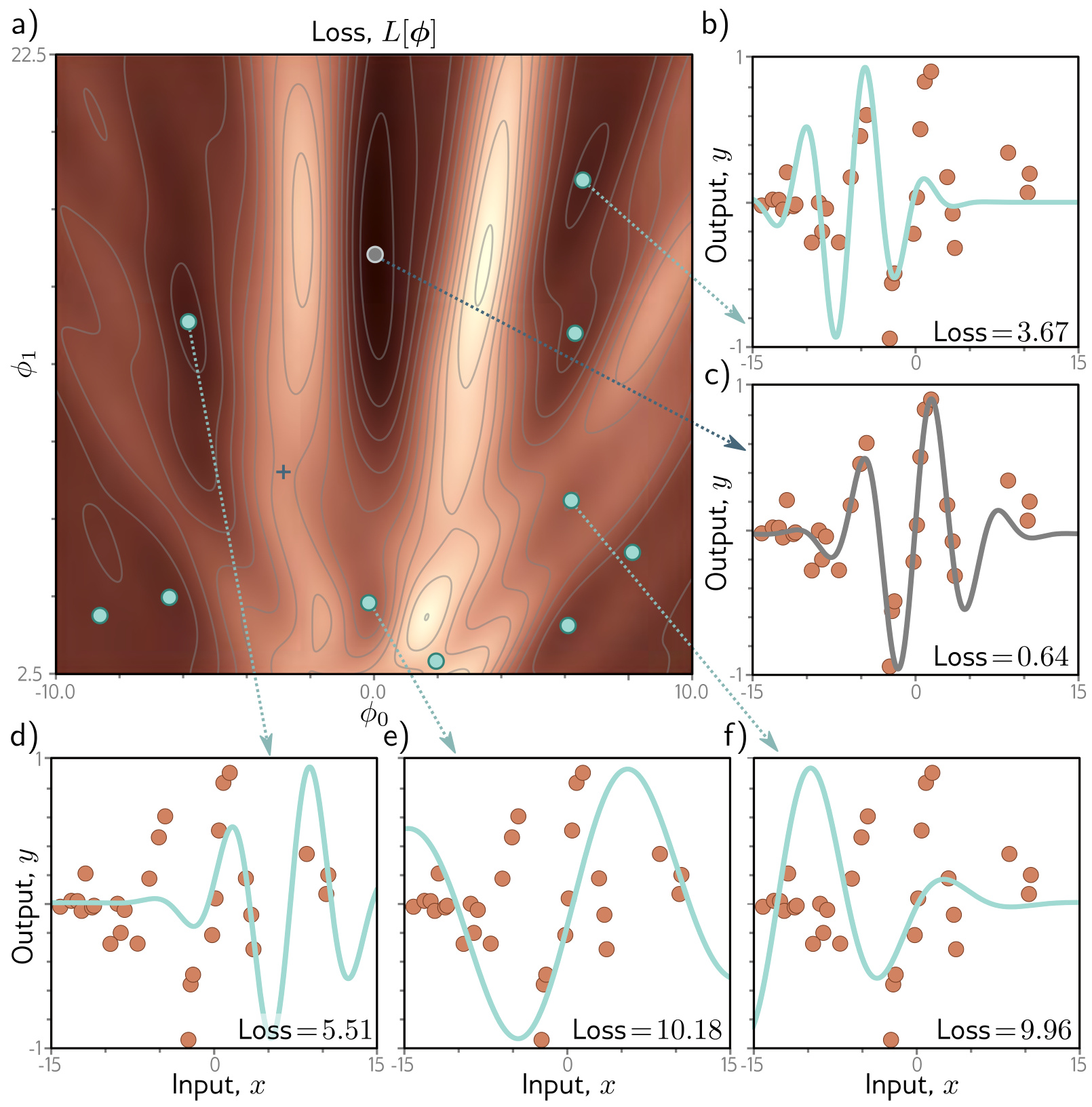
A non-convex surface: the Gabor model
\[
\begin{aligned}
f[x,\phi] &= \sin[\phi_0 + 0.06\,\phi_1 x]\\
&\quad\cdot\exp\left(-\frac{(\phi_0+0.06\,\phi_1 x)^2}{32.0}\right)
\end{aligned}
\]
A sinusoid whose amplitude decays away from its centre
Two parameters, so the whole loss surface can be drawnTrained on 28 pairs from \(\phi = [0.0, 16.6]^T\) plus noise
What two parameters already cost
Cyan — local minima , losses \(3.67\) to \(10.18\)
Gray — the global minimum , loss \(0.64\)
Blue cross — a saddle point
Where descent lands is decided by where it started.
Local minima and saddle points
Local minimum
Gradient zero
Loss increases in every direction
Not the overall minimum
No small step improves it
Saddle point
Gradient zero
Increases in some directions
Decreases in others
Descent escapes — but slowly
Near a saddle the surface is flat, so a small-gradient stopping rule stops there.
Higher dimensions make it worse
Two parameters can be searched exhaustively, or restarted from many positions
A network has millions of parameters, and neither is possible
Every additional dimension adds directions along which the surface can be flat
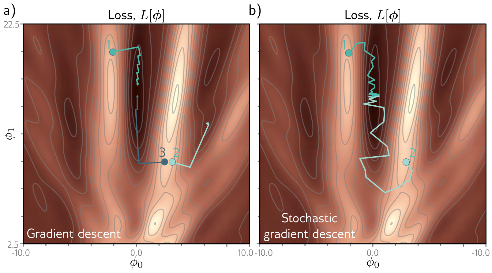
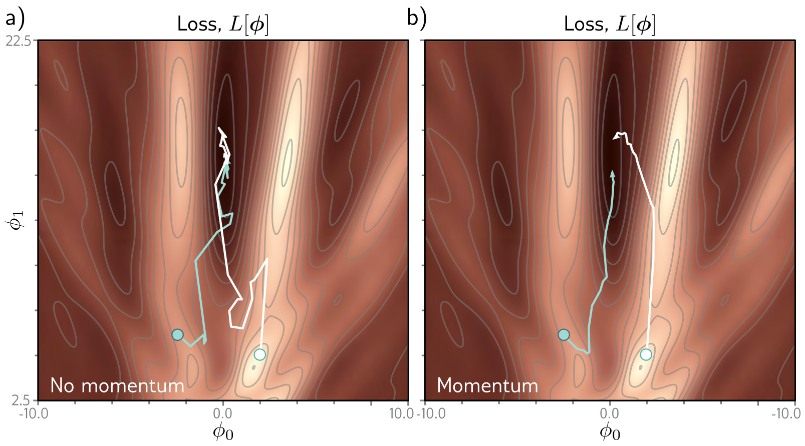
The destination of a descent run is determined entirely by its starting point.
This is what motivates every modification that follows. Not a better downhill rule, but noise in the direction, so that the starting point stops being decisive.
Momentum
\[
\begin{aligned}
m_{t+1} &\leftarrow \beta\cdot m_t + (1-\beta)\sum_{i\in\mathcal{B}_t}\frac{\partial \ell_i[\phi_t]}{\partial\phi}\\
\class{hg-key}{\phi_{t+1}} &\class{hg-key}{{}\leftarrow \phi_t - \alpha\cdot m_{t+1}}
\end{aligned}
\]
The step is a weighted combination of this batch’s gradient and the direction moved last.
What momentum does
The recursion makes the step an infinite weighted sum of past gradients
Weights shrink as one moves back in time
Aligned gradients
Terms add , so the effective learning rate rises.
Oscillating gradients
Terms cancel , so the effective rate falls.
Smoother trajectory, less oscillation in valleys.
A fixed step size is misallocated
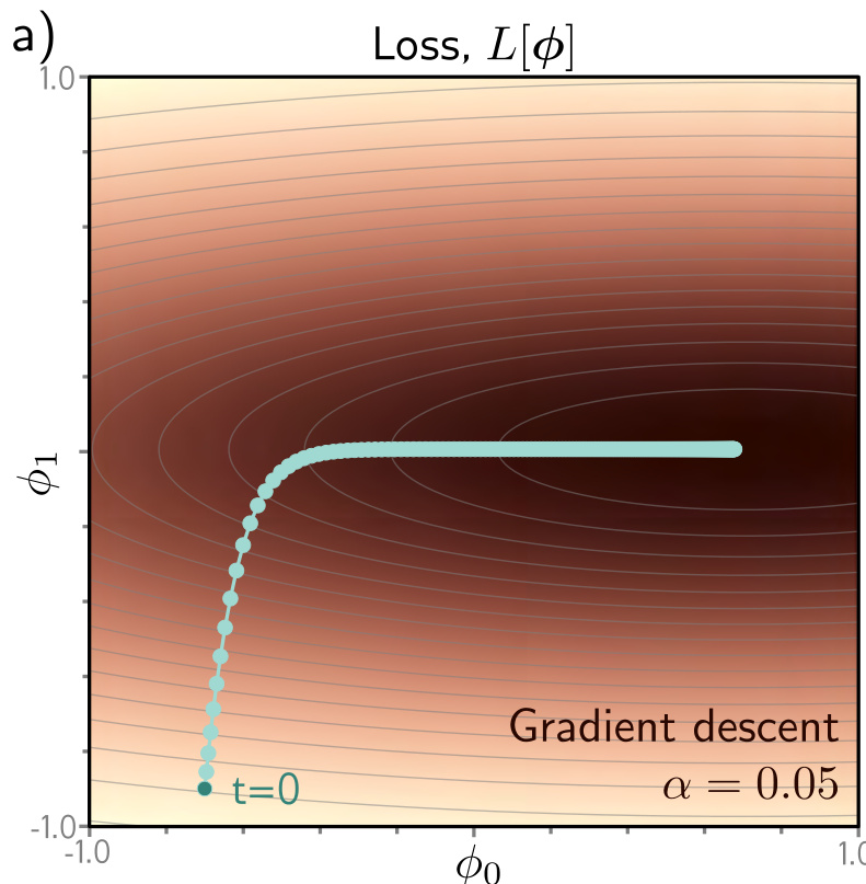
\(\alpha = 0.05\) : stable, and very slow.
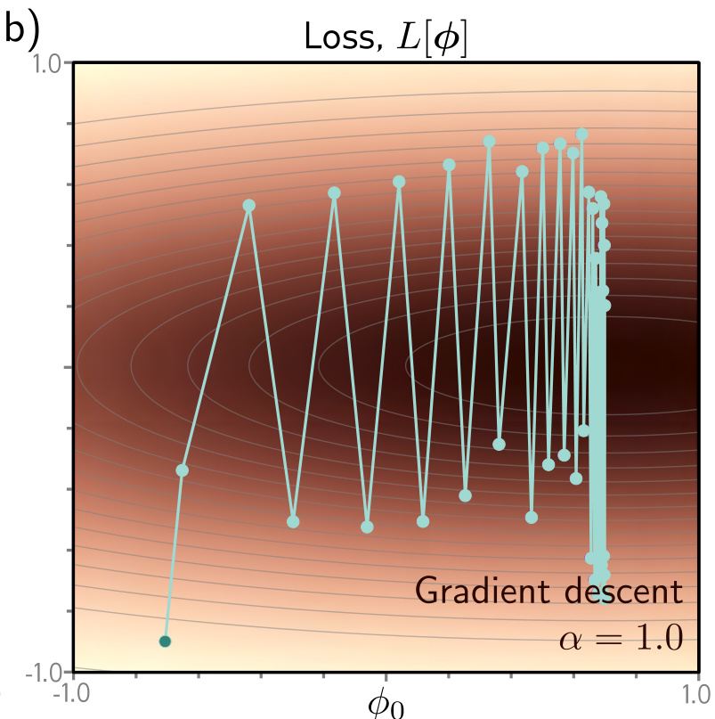
\(\alpha = 1.0\) : fast, and unstable.
No single rate suits a surface steeper in one direction than another.
Normalizing the gradient
Measure the gradient and its pointwise square:
\[m_{t+1} \leftarrow \frac{\partial L[\phi_t]}{\partial\phi}, \qquad v_{t+1} \leftarrow \left(\frac{\partial L[\phi_t]}{\partial\phi}\right)^2\]
then divide one by the root of the other:
\[\class{hg-key}{\phi_{t+1} \leftarrow \phi_t - \alpha\cdot\frac{m_{t+1}}{\sqrt{v_{t+1}}+\epsilon}}\]
Why the normalizing factor
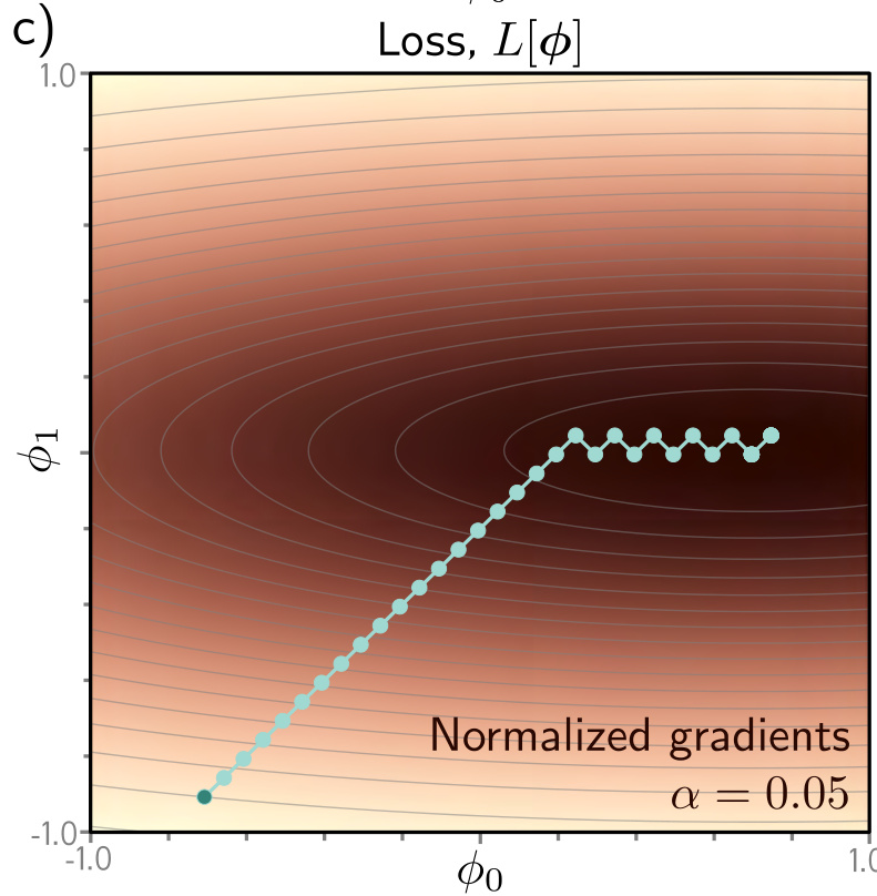
Normalized gradients, \(\alpha = 0.05\) .
Only the sign survives in each coordinate
So each moves a fixed distance \(\alpha\) downhill
Good progress in both directions
But it bounces around the minimum
Adam
\[
\begin{aligned}
m_{t+1} &\leftarrow \beta m_t + (1-\beta)\frac{\partial L}{\partial\phi}\\
v_{t+1} &\leftarrow \gamma v_t + (1-\gamma)\left(\frac{\partial L}{\partial\phi}\right)^2
\end{aligned}
\]
Early estimates start from zero, so correct them:
\[\tilde{m}_{t+1} \leftarrow \frac{m_{t+1}}{1-\beta^{t+1}}, \qquad \tilde{v}_{t+1} \leftarrow \frac{v_{t+1}}{1-\gamma^{t+1}}\]
The correction terms
\[\class{hg-key}{\phi_{t+1} \leftarrow \phi_t - \alpha\cdot\frac{\tilde{m}_{t+1}}{\sqrt{\tilde{v}_{t+1}}+\epsilon}}\]
\(\beta, \gamma \in [0,1)\) , so \(\beta^{t+1}\) and \(\gamma^{t+1}\) shrink each stepThe denominators approach one, and the correction fades
It matters only for the first few iterations
The hyperparameters
\(\alpha\) — the learning rate\(\beta\) — momentum on the gradient, typically \(0.9\) \(\gamma\) — momentum on the squared gradient, typically \(0.99\) \(\epsilon\) — a small constant preventing division by zero
Adam is less sensitive to the initial learning rate , so it needs no elaborate schedule.
Adam is the robust choice
Gradient magnitudes depend on a parameter’s depth in the network
Adam compensates, balancing changes across layers
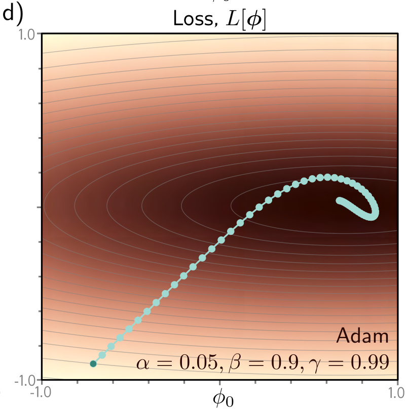
\(\alpha = 0.05\) , \(\beta = 0.9\) , \(\gamma = 0.99\)
The trajectory, smoothed
SGD, with and without momentum.
Adam: momentum on both terms.
In practice both statistics come from minibatches, so the real path is noisier.
What the optimisers assumed
For a network with three hidden layers,
\[
\begin{aligned}
h_1 &= a[\beta_0 + \Omega_0 x], & h_2 &= a[\beta_1 + \Omega_1 h_1],\\
h_3 &= a[\beta_2 + \Omega_2 h_2], & f[x,\phi] &= \beta_3 + \Omega_3 h_3
\end{aligned}
\]
every update needs \(\partial\ell_i/\partial\beta_k\) and \(\partial\ell_i/\partial\Omega_k\) for every layer — at every iteration, for models of \(10^{12}\) parameters.
Two observations
Observation 1
A weight’s effect is scaled by the activation at its source .
So store every activation on the way forward — the forward pass .
Observation 2
A change ripples through every later layer.
The same quantities recur, so compute them once, in reverse — the backward pass .
The toy example
Eight scalar parameters, composing \(\sin\) , \(\exp\) and \(\cos\) :
\[
\begin{aligned}
h &= \sin[\beta_0+\omega_0 x]\\
f[x,\phi] &= \beta_3 + \omega_3\cos\big[\beta_2 + \omega_2\exp[\beta_1+\omega_1 h]\big]
\end{aligned}
\]
Differentiating by hand is possible but error-prone
And wasteful: \(\partial\ell_i/\partial\omega_0\) repeats the same exponential three times
The forward pass
\[
\begin{aligned}
f_0 &= \beta_0 + \omega_0 x_i, & h_1 &= \sin[f_0],\\
f_1 &= \beta_1 + \omega_1 h_1, & h_2 &= \exp[f_1],\\
f_2 &= \beta_2 + \omega_2 h_2, & h_3 &= \cos[f_2],\\
f_3 &= \beta_3 + \omega_3 h_3, & \ell_i &= (f_3 - y_i)^2
\end{aligned}
\]
Every intermediate value is computed once and kept.
The parameter derivatives
The chain rule expresses each parameter derivative in terms of the derivative at its own pre-activation, \(\partial\ell_i/\partial f_k\) :
\[\frac{\partial\ell_i}{\partial\beta_k} = \frac{\partial f_k}{\partial\beta_k}\frac{\partial\ell_i}{\partial f_k}, \qquad \frac{\partial\ell_i}{\partial\omega_k} = \frac{\partial f_k}{\partial\omega_k}\frac{\partial\ell_i}{\partial f_k}\]
Since \(f_k = \beta_k + \omega_k h_k\) , the two local terms are immediate:
\[\frac{\partial f_k}{\partial\beta_k} = 1, \qquad \frac{\partial f_k}{\partial\omega_k} = h_k\]
The eight parameter derivatives reduce to the four \(\partial\ell_i/\partial f_k\) , which the backward pass computes.
The backward pass
Start at the end, \(\partial\ell_i/\partial f_3 = 2(f_3-y_i)\) , then chain backwards:
\[\frac{\partial\ell_i}{\partial f_2} = \frac{\partial h_3}{\partial f_2}\left(\frac{\partial f_3}{\partial h_3}\frac{\partial\ell_i}{\partial f_3}\right)\]
The bracketed term was computed at the previous step.
From scalars to layers
The toy example used scalar weights. In a real network each \(\omega_k\) becomes a matrix \(\Omega_k\) and each \(f_k\) a vector:
\[f_0 = \beta_0 + \Omega_0 x_i, \qquad h_k = a[f_{k-1}], \qquad f_k = \beta_k + \Omega_k h_k\]
The backward step carries the same structure, with a transpose where the scalar had none:
\[\frac{\partial\ell_i}{\partial\Omega_k} = \frac{\partial\ell_i}{\partial f_k}h_k^T, \qquad \frac{\partial\ell_i}{\partial f_{k-1}} = \mathbb{I}[f_{k-1}>0]\odot\left(\Omega_k^T\frac{\partial\ell_i}{\partial f_k}\right)\]
Forward multiplies by \(\Omega_k\) ; backward multiplies by \(\Omega_k^T\) .
The activation derivative appears as the indicator, since a ReLU passes the incoming derivative where its input was positive and blocks it elsewhere. Every example in the batch is treated this way and the results are summed for the SGD update.
Cheap in time, expensive in memory
The cost
One matrix multiply per pass
\(\Omega_k\) forward, \(\Omega_k^T\) backEvery activation stored until the backward pass
When it does not fit
Checkpointing — keep some, recompute the restDistributed — split by batch, layer or operation
Memory, not arithmetic, caps the model size.
Algorithmic differentiation
Frameworks derive the gradients from the model specification alone.
Each component knows its own derivative
The framework knows the order of operations
Together: both passes, with nothing coded by hand
Batches run in parallel, the input a tensor
Nothing requires the network to be sequential. The ideas hold for any acyclic computational graph, which is what PyTorch and TensorFlow support.
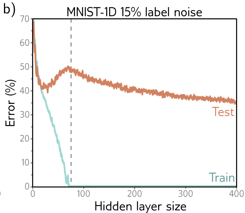
Perfect training, poor test
MNIST-1D — ten classes, \(I = 4000\) examples, \(D_i = 40\) dimensions.
Two hidden layers of \(D = 100\) , softmax over \(D_o = 10\)
SGD, batch 100, learning rate \(0.1\) , 6000 steps
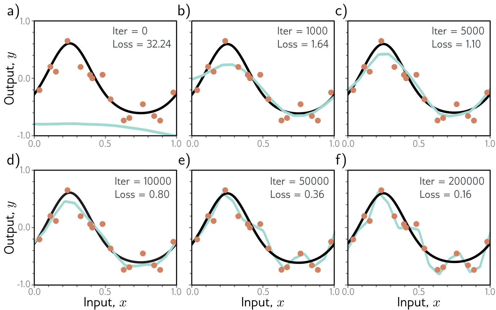
Training data classified perfectly by about 4000 steps
Test error on 1000 fresh examples: about 40%
Chance is 90%, so it learned — but it also memorised
The test loss rises
Test error falls, then flattens
Test loss falls for 1500 steps, then climbs
The model makes the same mistakes with growing confidence. The softmax drives pre-softmax activations to extremes, so the negative log-likelihood grows while the error rate does not.
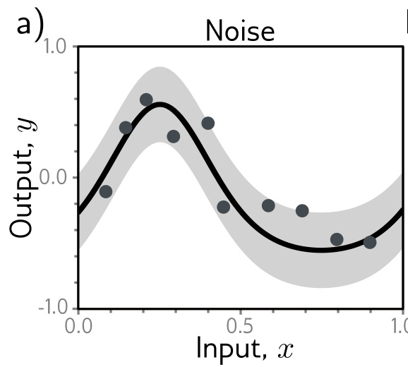
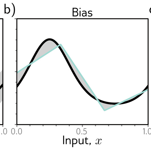
Noise and bias
Noise — several valid \(y\) per \(x\) .
Bias — the family cannot fit the truth.
Noise limits the test set, not the training set — the same \(x\) rarely recurs.
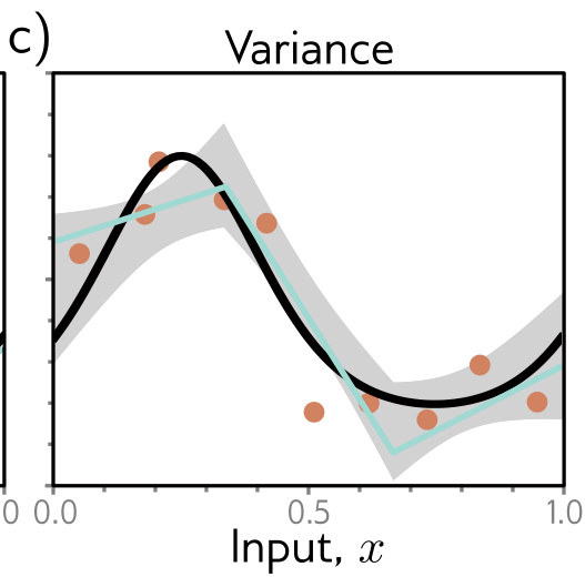
Variance
The training examples are limited
Noise cannot be told from signal
A different sample gives a different fit
A stochastic optimizer adds more.
Two averages
The truth
\[\mu[x] = \mathbb{E}_y\big[y[x]\big]\]
The mean of \(Pr(y|x)\) , averaged over the noise.
The model
\[f_\mu[x] = \mathbb{E}_\mathcal{D}\Big[f\big[x,\phi[\mathcal{D}]\big]\Big]\]
The fitted function, averaged over training sets \(\mathcal{D}\) .
Bias is the gap between them; variance is the spread about \(f_\mu[x]\) .
The decomposition
\[
\begin{aligned}
\mathbb{E}_\mathcal{D}\Big[\mathbb{E}_y\big[L[x]\big]\Big]
&= \underbrace{\mathbb{E}_\mathcal{D}\Big[\big(f[x,\phi[\mathcal{D}]]-f_\mu[x]\big)^2\Big]}_{\text{variance}}\\
&+ \underbrace{\big(f_\mu[x]-\mu[x]\big)^2}_{\text{bias}}
+ \underbrace{\sigma^2}_{\text{noise}}
\end{aligned}
\]
The three combine additively for least-squares regression
The cross terms vanish, each containing a mean minus its own expectation
What to change
Variance
Reduced by more data — noise averages out and the input space is better sampled.
Bias
Reduced by more capacity — hidden units or layers the model can use.
Noise admits no remedy. It is the floor.
The bias-variance trade-off
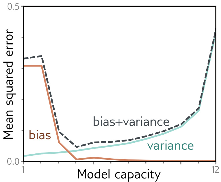
Bias (orange) falls with capacity
Variance (cyan) rises
Their sum is least at capacity four
Ten regions fit fifteen points better than three — but the extra power models the noise.