Lecture notes — Early Object Detection Networks
Keywords
ver. 1.1.6, early_object_detection_networks
← Early Object Detection Networks
ver. 1.1.6 · 2026-10-02 01:11:15
Where this fits
The previous unit, Residual Convolutional Networks, produced backbones that train at great depth — ResNet, DenseNet, SqueezeNet, MobileNet — and each of them answers one question about a whole image: which class is it? Detection asks for a variable-length list of boxes, each with a label and a score, and grades an answer by spatial overlap rather than by equality. The backbones carry over unchanged; what changes is everything attached to them, and the three papers of this unit remove one hand-built component after another until the detector is a single network trained by stochastic gradient descent.
Learning outcomes
detection-task-and-evaluation— State the object detection problem and evaluate a detector with IoU-based mean average precision.region-proposal-pipeline— Describe the R-CNN pipeline: category-independent proposals, CNN features on warped regions, class-specific SVMs.transfer-learning-for-detection— Adapt an ImageNet-pre-trained CNN to detection by domain-specific fine-tuning, and justify the label and classifier choices.bounding-box-regression— Apply bounding-box regression to refine proposals and read a detection error analysis.roi-pooling-shared-computation— Explain how RoI pooling lets all proposals share one convolutional forward pass.multi-task-loss-and-single-stage-training— Train a detector in one stage with a multi-task classification and localisation loss.rpn-and-anchors— Design a Region Proposal Network with translation-invariant anchor boxes.feature-sharing-training— Train an RPN and a Fast R-CNN detector so that they share one set of convolutional features.compare-detector-generations— Compare R-CNN, Fast R-CNN and Faster R-CNN on accuracy and speed, and name the bottleneck each removed.
Concepts introduced
- R-CNN (Regions with CNN features) — detection performed by classifying about 2000 category-independent region proposals with CNN features and per-class linear SVMs.
- Region proposal warping and context padding — a proposal is dilated by \(p = 16\) pixels of context and anisotropically warped to the network’s fixed \(227 \times 227\) input.
- Supervised pre-training and domain-specific fine-tuning — the CNN is trained on ILSVRC image-level labels, then fine-tuned by SGD on warped detection proposals.
- Bounding-box regression — a class-specific linear model on \(\text{pool}_5\) features maps a proposal to a nearby ground-truth box.
- Non-parametric unit feature visualisation — a single \(\text{pool}_5\) unit is ranked over millions of held-out proposals to show what it detects.
- Region of interest (RoI) pooling — an \(h \times w\) window on a shared convolutional feature map is max-pooled into a fixed \(H \times W\) grid.
- Multi-task loss — classification and localisation are optimised together in one training stage.
- Smooth \(L_1\) loss — a localisation loss quadratic near zero and linear beyond it.
- Hierarchical mini-batch sampling — a mini-batch draws few images and many RoIs from each, so RoIs share a forward and backward pass.
- Truncated SVD compression — a fully connected weight matrix is factorised at rank \(t\) to cut test-time cost.
- Region Proposal Network (RPN) — a small fully convolutional network over the shared feature map that emits objectness scores and box offsets.
- Anchor boxes — \(k\) reference boxes of several scales and aspect ratios at every sliding-window position.
- RPN multi-task loss — objectness log loss plus a smooth \(L_1\) box loss over sampled anchors.
- 4-step alternating training — a four-stage recipe that ties the convolutional layers of an RPN and a detector together.
- Faster R-CNN — an RPN and a Fast R-CNN detector as one network over shared convolutions.
From classification to detection
A classifier maps an image to one of \(N\) labels. A detector must output a list of rectangles, each carrying a class label and a confidence score, and the list length varies with the image. Correctness is graded by intersection over union, the ratio of the area shared by two boxes to the area their union covers,
\[\mathrm{IoU}(A, B) = \frac{|A \cap B|}{|A \cup B|},\]
so a predicted box counts as a true positive when its IoU with a ground-truth box of the same class is at least \(0.5\). Ranking all predictions of one class by score gives a precision-recall curve and hence an average precision; the mean average precision (mAP) is that quantity averaged over classes. It is the number every result in this unit reports.
The detection error analysis of Girshick et al., “Rich feature hierarchies for accurate object detection and semantic segmentation”, counts a box whose IoU with the correct class lies between \(0.1\) and \(0.5\) as a localisation false positive, which is a useful reading of what the \(0.5\) threshold excludes.
Two ways of adapting a classification network to this task were available and both fail at depth.
Localisation as regression from the image to box coordinates.
Szegedy et al., working concurrently, report \(30.5\%\) mAP on VOC 2007 by this route, against the \(58.5\%\) that Girshick et al. reach on the same data.
Localisation by a sliding window over a dense grid of positions.
Girshick et al. note that units high in their network — five convolutional layers deep — have receptive fields of \(195 \times 195\) pixels and strides of \(32 \times 32\) pixels in the input image, which makes precise localisation inside the sliding-window paradigm an open problem.
The third difficulty is data. Detection annotation is scarce beside ImageNet classification annotation, so a high-capacity network cannot be trained for detection from scratch; the classifier that already exists has to be reused. The three papers answer these problems in sequence, and each generation’s contribution is best stated as the bottleneck it removed: per-proposal convolution, then multi-stage training, then the externally computed proposals.
NoteOutcomes and concepts
Learning outcomes
- detection-task-and-evaluation State the object detection problem and evaluate a detector with IoU-based mean average precision.
- compare-detector-generations Compare R-CNN, Fast R-CNN and Faster R-CNN on accuracy and speed, and name the bottleneck each removed.
The R-CNN pipeline
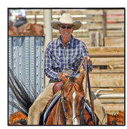
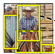
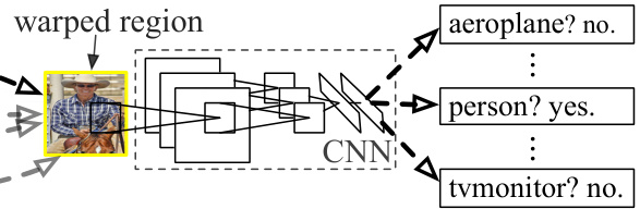
Girshick et al., “Rich feature hierarchies for accurate object detection and semantic segmentation”, solve localisation by working in the recognition using regions paradigm. R-CNN consists of three modules: one that generates category-independent region proposals, one large convolutional network that extracts a fixed-length feature vector from each region, and a set of class-specific linear SVMs.
Region proposals
The method is agnostic to the proposal algorithm — objectness, selective search, CPMC and multi-scale combinatorial grouping are all listed as candidates — and selective search in its “fast mode” is used to permit a controlled comparison with prior work. It emits around 2000 candidate boxes per image.
Feature extraction
The network requires a fixed \(227 \times 227\) input, and proposals are arbitrary rectangles. Of the possible transformations the simplest is taken: anisotropic warping with context padding. All pixels in a tight bounding box around the proposal are warped to the required size, and before warping the box is dilated so that exactly \(p = 16\) pixels of warped image context surround the original box. Where the source rectangle extends past the image, the missing data is replaced with the image mean. A 4096-dimensional feature vector is then computed by forward propagating the mean-subtracted region through five convolutional and two fully connected layers.
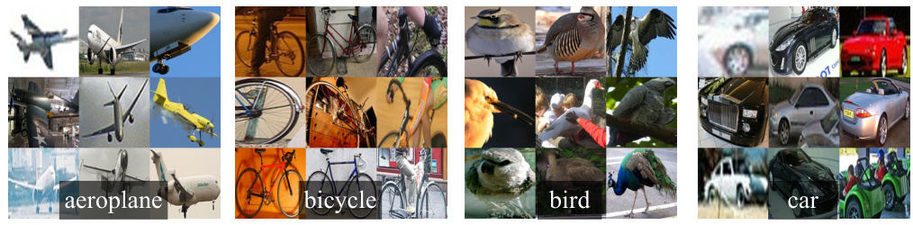
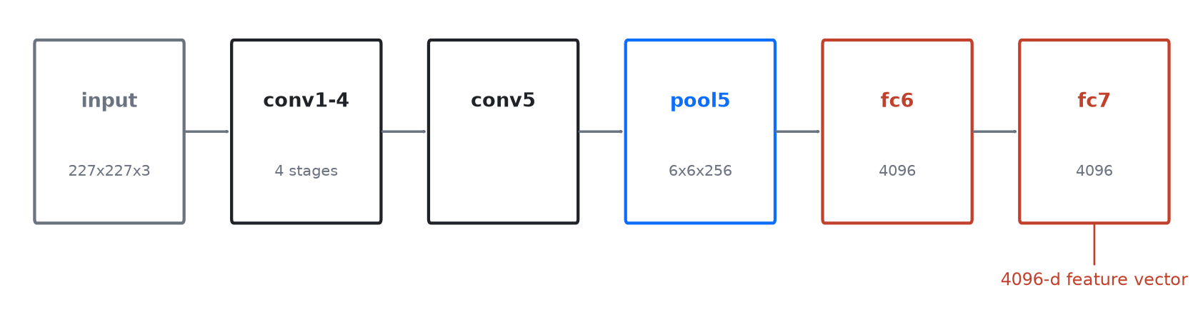
The network those regions pass through is the Krizhevsky architecture, called T-Net in the paper: five convolutional stages, the last of them pooled, followed by two fully connected layers. Each named layer below is referred to by that name throughout the rest of this unit.
Appendix A of the paper compares this warp against enclosing each proposal in the tightest square with context and in the tightest square without context. Warping with \(p = 16\) pixels of context padding outperformed the alternatives by 3 to 5 mAP points.
Classification and suppression
Each feature vector is scored by the linear SVM trained for each class. Across all scored regions in an image, a greedy non-maximum suppression, run independently per class, rejects a region if it has an IoU overlap with a higher-scoring selected region larger than a learned threshold.
Stated precisely, for one class let \(\mathcal{B} = \{(b_i, s_i)\}_{i=1}^{M}\) be the scored regions, where \(b_i\) is a box and \(s_i\) its SVM score, and let
\[\operatorname{IoU}(b, b') = \frac{|b \cap b'|}{|b \cup b'|}\]
be the intersection over union of two boxes. Non-maximum suppression at threshold \(\tau\) returns the set \(\mathcal{D}\) produced by iterating
\[ \begin{aligned} m &\leftarrow \operatorname*{argmax}_{i \,:\, (b_i, s_i) \in \mathcal{B}} s_i,\\ \mathcal{D} &\leftarrow \mathcal{D} \cup \{b_m\},\\ \mathcal{B} &\leftarrow \mathcal{B} \setminus \big(\{(b_m, s_m)\} \cup \{(b_i, s_i) : \operatorname{IoU}(b_m, b_i) > \tau\}\big), \end{aligned} \]
until \(\mathcal{B}\) is empty, starting from \(\mathcal{D} = \emptyset\). Each pass takes the highest-scoring surviving box, keeps it, and discards every box overlapping it by more than \(\tau\). The procedure is greedy in that a box once kept is never reconsidered, and it is run separately per class, so two boxes of different classes never suppress each other.
Two properties make this efficient. All CNN parameters are shared across categories, so the 13 s per image on a GPU (53 s on a CPU) spent computing proposals and features is amortised over every class. And the only class-specific computation is a matrix product: a \(2000 \times 4096\) feature matrix against a \(4096 \times N\) matrix of SVM weights, followed by non-maximum suppression. At 100k classes that multiplication takes 10 seconds on a multi-core CPU and 1.5 GB of memory, where the 360k-dimensional features of the UVA system would need 134 GB.
The cost that matters is the 2000 forward passes. Nothing in the pipeline is shared between two proposals that overlap by 90%, and the whole of the engineering in the next two papers follows from that.
NoteOutcomes and concepts
Learning outcomes
- detection-task-and-evaluation State the object detection problem and evaluate a detector with IoU-based mean average precision.
- region-proposal-pipeline Describe the R-CNN pipeline: category-independent proposals, CNN features on warped regions, class-specific SVMs.
Concepts
- r-cnn three modules — category-independent proposals, a CNN feature extractor, and per-class linear SVMs — turn detection into region classification
- region-proposal-warping a proposal is dilated by \(p = 16\) pixels of context and anisotropically warped to \(227 \times 227\), which beats square crops by 3 to 5 mAP points
Pre-training, fine-tuning and the SVMs
Supervised pre-training runs first: the CNN is discriminatively trained on the ILSVRC2012 classification set using image-level annotations only, with no bounding boxes available. Domain-specific fine-tuning then adapts it to the new task and the new domain of warped proposal windows. The ImageNet 1000-way classification layer is replaced by a randomly initialised \((N+1)\)-way layer — \(N\) object classes plus background, so \(N = 20\) for VOC and \(N = 200\) for ILSVRC2013 — and the architecture is otherwise unchanged. SGD continues at a learning rate of \(0.001\), one tenth of the initial pre-training rate, which lets fine-tuning make progress without clobbering the initialisation. Each mini-batch of 128 is built from 32 positive windows sampled uniformly over all classes and 96 background windows, a deliberate bias towards positives because they are extremely rare beside background.
Two definitions of a positive
For fine-tuning, a proposal is positive for the class of the ground-truth instance with which it has maximum IoU, provided that IoU is at least \(0.5\); everything else is background. For SVM training the definition is stricter: only ground-truth boxes are positive, proposals overlapping an instance by less than \(0.3\) IoU are negative for that class, and proposals in the grey zone between are simply ignored. The \(0.3\) threshold was selected by grid search over \(\{0, 0.1, \ldots, 0.5\}\) on a validation set, and the choice matters — setting it to \(0.5\) cost 5 mAP points and setting it to \(0\) cost 4.
ImportantThe two thresholds are not an inconsistency
Appendix B gives the reason. Fine-tuning has too little data, and the relaxed definition supplies roughly 30 times as many positive examples in the form of jittered windows, which is what allows the entire network to be fine-tuned without overfitting. The cost is that those jittered examples do not emphasise precise localisation. SVM training does not need the extra data, so it uses the exact positives instead, together with standard hard negative mining, which converges after a single pass over the images.
Applying the fine-tuned 21-way softmax directly as the detector drops VOC 2007 performance from \(54.2\%\) to \(50.9\%\) mAP. The gap is attributed to the jittered positive definition and to the softmax classifier being trained against randomly sampled negatives rather than the hard negatives the SVMs see.
Where the representation lives
The three layers compared here are the last three of the T-Net feature extractor above, and the names are that network’s: \(\text{pool}_5\) is the pooled output of the fifth and final convolutional stage, a \(6 \times 6 \times 256\) map; \(\text{fc}_6\) and \(\text{fc}_7\) are the two fully connected layers stacked on it, each producing 4096 dimensions. The detector reads whichever of the three is named, discarding everything above it.
Without fine-tuning, the layer-by-layer results on VOC 2007 are \(44.2\%\) mAP from \(\text{pool}_5\), \(46.2\%\) from \(\text{fc}_6\) and \(44.7\%\) from \(\text{fc}_7\). Features from \(\text{fc}_7\) generalise worse than those from \(\text{fc}_6\), meaning that \(29\%\) of the network’s parameters — some 16.8 million — can be removed without degrading mAP, and \(\text{pool}_5\) alone performs well using only \(6\%\) of the parameters. Fine-tuning raises mAP by 8.0 points to \(54.2\%\), and the boost is much larger for \(\text{fc}_6\) and \(\text{fc}_7\) than for \(\text{pool}_5\): the convolutional features transfer from ImageNet largely intact, and what fine-tuning learns is the domain-specific non-linear classifier stacked on them.
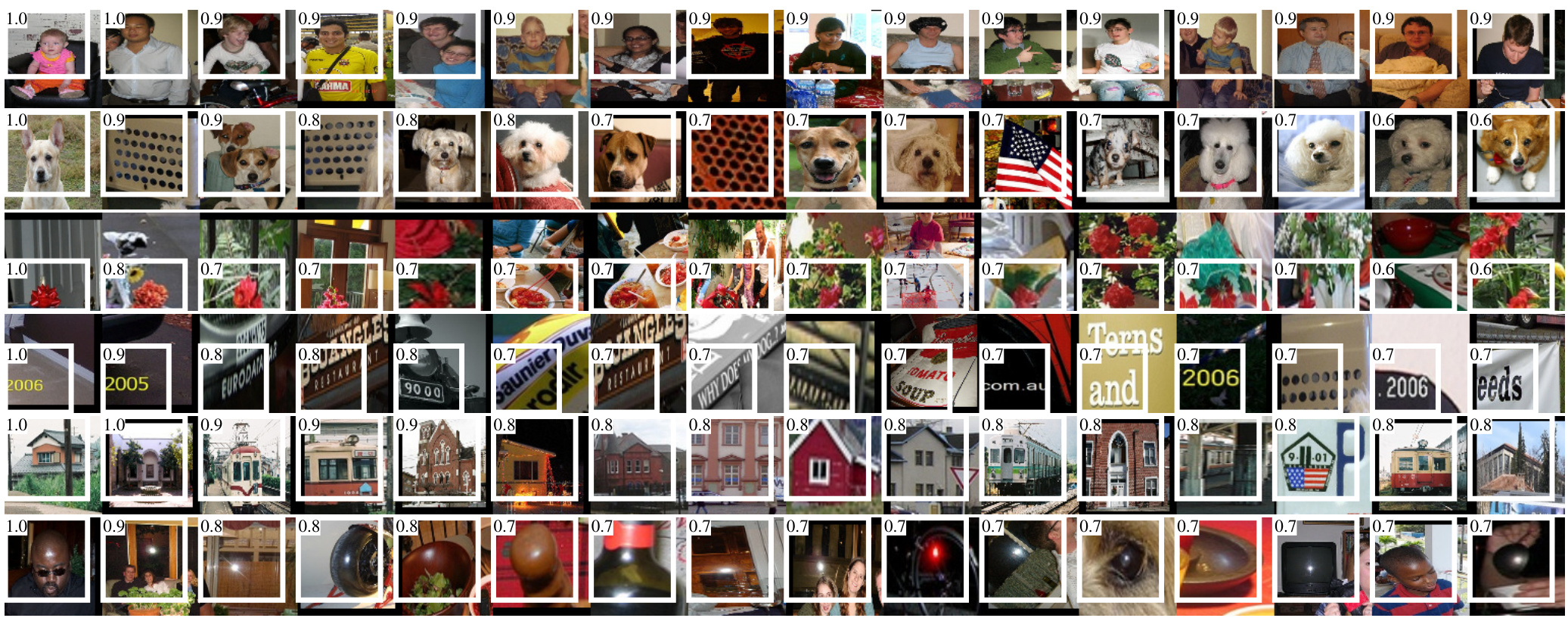
Non-parametric unit feature visualisation shows what those convolutional features are. The \(\text{pool}_5\) map is \(6 \times 6 \times 256 = 9216\)-dimensional and each unit has a receptive field of \(195 \times 195\) pixels in the input. Treating one unit as a detector in its own right, its activations are computed over about 10 million held-out proposals, sorted from highest to lowest, put through non-maximum suppression, and the top-scoring regions displayed. No averaging is done, so distinct visual modes remain visible.
NoteOutcomes and concepts
Learning outcomes
- transfer-learning-for-detection Adapt an ImageNet-pre-trained CNN to detection by domain-specific fine-tuning, and justify the label and classifier choices.
- region-proposal-pipeline Describe the R-CNN pipeline: category-independent proposals, CNN features on warped regions, class-specific SVMs.
Concepts
- supervised-pre-training-domain-fine-tuning pre-training on ILSVRC2012 image-level labels followed by SGD on warped proposals is worth 8.0 mAP points, concentrated in the fully connected layers
- r-cnn the three modules are trained in three separate stages, and the SVM stage outperforms the fine-tuned softmax by 3.3 mAP
- feature-visualization-nonparametric ranking one \(\text{pool}_5\) unit over about 10 million held-out proposals, without averaging, shows the visual modes that unit responds to
Localisation error and bounding-box regression
The diagnostic tool of Hoiem et al. sorts a detector’s top-ranked false positives into four types: Loc, a detection with an IoU overlap with the correct class between \(0.1\) and \(0.5\), or a duplicate; Sim, confusion with a similar category; Oth, confusion with a dissimilar category; and BG, a false positive fired on background.
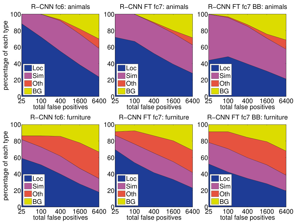
Significantly more of R-CNN’s errors are Loc than are BG or other-class confusions, the reverse of the pattern DPM shows. The conclusion is that the CNN features are far more discriminative than HOG, and that the loose localisation left over comes from the proposal boundaries and from the positional invariance the network learned while being pre-trained for whole-image classification.
The regressor
Bounding-box regression removes that error. The training input is a set of pairs \(\{(P^i, G^i)\}_{i=1,\ldots,N}\), where \(P = (P_x, P_y, P_w, P_h)\) gives the pixel coordinates of a proposal’s centre together with its width and height, and \(G\) is a ground-truth box in the same form. Four functions \(d_x(P)\), \(d_y(P)\), \(d_w(P)\), \(d_h(P)\) are learned, and a proposal is transformed into a predicted box \(\hat{G}\) by
\[\hat{G}_x = P_w d_x(P) + P_x, \qquad \hat{G}_y = P_h d_y(P) + P_y,\] \[\hat{G}_w = P_w \exp(d_w(P)), \qquad \hat{G}_h = P_h \exp(d_h(P)).\]
The first two are a scale-invariant translation of the centre and the second two are log-space translations of the width and height. The regression targets that fit them are
\[t_x = (G_x - P_x)/P_w, \quad t_y = (G_y - P_y)/P_h, \quad t_w = \log(G_w/P_w), \quad t_h = \log(G_h/P_h).\]
Each \(d_\star(P) = \mathbf{w}_\star^{\mathrm{T}} \boldsymbol{\phi}_5(P)\) is a linear function of the \(\text{pool}_5\) features of the proposal, and \(\mathbf{w}_\star\) is learned by regularised least squares — ridge regression:
\[\mathbf{w}_\star = \operatorname*{argmin}_{\hat{\mathbf{w}}_\star} \sum_i^N \big(t^i_\star - \hat{\mathbf{w}}_\star^{\mathrm{T}} \boldsymbol{\phi}_5(P^i)\big)^2 + \lambda \|\hat{\mathbf{w}}_\star\|^2 .\]
ImportantTwo implementation details the paper flags
Regularisation is important: \(\lambda = 1000\) was chosen on a validation set. And the training pairs must be selected with care. Transforming a \(P\) that lies far from every ground-truth box into some \(G\) is not a well-posed problem, so a proposal is used only if it is nearby — assigned to the \(G\) with which it has maximum IoU, and only if that overlap exceeds \(0.6\). Unassigned proposals are discarded. This is done once per class, giving class-specific regressors.
At test time the transform is applied once to each scored proposal. Iterating the procedure — re-scoring the predicted box, predicting again — was tried and does not improve results. The single application is worth 3 to 4 mAP points: VOC 2007 rises from \(54.2\%\) to \(58.5\%\) and VOC 2010 from \(50.2\%\) to \(53.7\%\).
The pattern established here is the one the rest of the unit repeats. Measure where the errors are, then add the cheapest module that removes them. The parameterisation \((t_x, t_y, t_w, t_h)\) reappears unchanged in Fast R-CNN and in the RPN.
NoteOutcomes and concepts
Learning outcomes
- bounding-box-regression Apply bounding-box regression to refine proposals and read a detection error analysis.
- detection-task-and-evaluation State the object detection problem and evaluate a detector with IoU-based mean average precision.
Concepts
- bounding-box-regression a class-specific ridge regression on \(\text{pool}_5\) features, fitted only on proposals overlapping a ground-truth box by more than \(0.6\) IoU, recovers 3 to 4 mAP points lost to mislocalisation
What R-CNN achieved, and what it cost
On VOC 2010 test, R-CNN reaches \(50.2\%\) mAP and \(53.7\%\) with bounding-box regression, against \(40.4\%\) for SegDPM, \(35.1\%\) for the UVA system that uses the same selective search proposals, and \(33.4\%\) for DPM v5. On VOC 2011/12 test it reaches \(53.3\%\).
The backbone matters as much as the pipeline. Substituting the 16-layer network of Simonyan and Zisserman — 13 layers of \(3 \times 3\) convolutions with five max pooling layers interspersed, topped by three fully connected layers, called O-Net in the paper — for the Krizhevsky architecture called T-Net raises VOC 2007 mAP from \(58.5\%\) to \(66.0\%\). Its forward pass takes roughly 7 times longer.
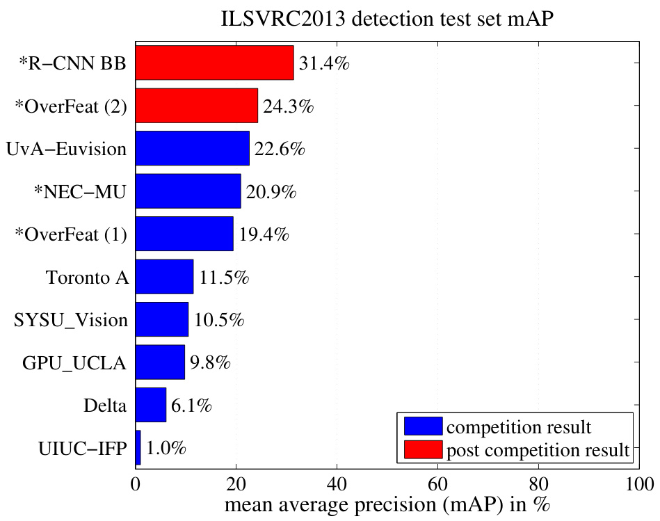
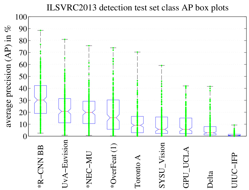
On the 200-class ILSVRC2013 detection set, run with the same system hyperparameters used for PASCAL VOC, R-CNN achieves \(31.4\%\) mAP against \(24.3\%\) for the post-competition OverFeat result, \(22.6\%\) for UvA-Euvision and \(20.9\%\) for NEC-MU.
The relationship to OverFeat
OverFeat can be seen, roughly, as a special case of R-CNN: replace the selective search proposals with a multi-scale pyramid of regular square regions and collapse the per-class bounding-box regressors into a single one, and the two systems become very similar. OverFeat is about \(9\times\) faster, at a quoted 2 seconds per image. The speed comes from the fact that its sliding windows are not warped at the image level, so computation can be shared between overlapping windows by running the network convolutionally over an arbitrarily sized input.
Evidence that the representation does the work
With minor modifications the same features transfer to semantic segmentation. Working inside the \(\text{O}_2\text{P}\) framework on 150 CPMC region proposals per image, three feature strategies are compared: full, the warped rectangle ignoring the region’s shape; fg, features computed on the foreground mask with the background replaced by the mean input; and full+fg, their concatenation. On VOC 2011 test, full+fg with \(\text{fc}_6\) gives \(47.9\%\) mean segmentation accuracy against \(40.8\%\) for Regions and Parts and \(47.6\%\) for \(\text{O}_2\text{P}\), and training its 20 support vector regressors takes an hour on one core rather than the ten or more hours \(\text{O}_2\text{P}\) needs.
Where the cost is
Girshick, “Fast R-CNN”, itemises what the design implies.
- Training is a multi-stage pipeline: fine-tune the network with log loss, fit SVMs to its features, then learn bounding-box regressors.
- Training is expensive in space and time. Features are extracted from every proposal in every image and written to disk; for VGG16 this takes 2.5 GPU-days for the 5k images of VOC07 trainval and requires hundreds of gigabytes of storage.
- Detection is slow. A VGG16 forward pass runs per proposal with no computation shared, taking 47 s per image on a GPU.
None of these is a defect in the implementation. Each is a consequence of classifying regions independently, and each is removed in turn by the papers that follow.
NoteOutcomes and concepts
Learning outcomes
- region-proposal-pipeline Describe the R-CNN pipeline: category-independent proposals, CNN features on warped regions, class-specific SVMs.
- compare-detector-generations Compare R-CNN, Fast R-CNN and Faster R-CNN on accuracy and speed, and name the bottleneck each removed.
Concepts
- r-cnn the region-based design reaches \(53.7\%\) mAP on VOC 2010 and \(31.4\%\) on ILSVRC2013, scales to a deeper backbone for \(66.0\%\) on VOC 2007, and transfers to segmentation
- bounding-box-regression every headline result quoted for R-CNN is the regressed one, and the regressor accounts for 3 to 4 points of it
Fast R-CNN and the RoI pooling layer
Spatial pyramid pooling networks had already shown that the convolutional feature map can be computed once for the whole image and each proposal classified from a vector max-pooled out of the shared map, accelerating R-CNN by 10 to \(100\times\) at test time and reducing training time by \(3\times\). The limitation was that the fine-tuning algorithm proposed for it cannot update the convolutional layers that precede the spatial pyramid pooling, and fixed convolutional layers limit the accuracy of very deep networks.
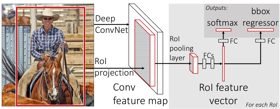
Fast R-CNN processes the whole image with several convolutional and max pooling layers to produce a conv feature map. An RoI — a region of interest — is a rectangular window on that map, defined by a four-tuple \((r, c, h, w)\) giving its top-left corner and its height and width. One RoI is one object proposal: the proposal arrives in image coordinates and is projected onto the feature map by dividing its coordinates by the network’s total stride, so a proposal of \(320 \times 480\) pixels becomes a window of about \(20 \times 30\) positions on a map at stride 16.
ImportantThe proposals still come from outside
Fast R-CNN removes the per-proposal forward pass, not the proposal step. It is trained and tested on pre-computed proposals from the same external candidate generator R-CNN used — selective search, around 2000 boxes per image — and the network takes a list of RoIs as a second input alongside the image. What changed is that those 2000 windows now index into one shared feature map instead of each demanding its own convolutional pass. The candidate generator is removed only in Faster R-CNN, where a Region Proposal Network computes the proposals from the same shared features.
The RoI pooling layer uses max pooling to convert the features inside any valid region of interest into a small feature map of fixed spatial extent \(H \times W\), where \(H\) and \(W\) are layer hyper-parameters independent of any particular RoI. That fixed output size is the whole purpose: the fully connected layers above it require a vector of fixed length, and proposals are arbitrary rectangles.
What the layer computes
Let \(\mathbf{X} \in \mathbb{R}^{C \times H' \times W'}\) be the conv feature map, with \(C\) channels, and let \((r, c, h, w)\) be an RoI on it. The \(h \times w\) window is divided into an \(H \times W\) grid of sub-windows, the \((i, j)\)-th of which covers the positions
\[ \mathcal{R}_{ij} = \left\{ (y, x) \;:\; \begin{aligned} r + \left\lfloor \tfrac{(i-1)h}{H} \right\rfloor &\le y < r + \left\lceil \tfrac{ih}{H} \right\rceil,\\ c + \left\lfloor \tfrac{(j-1)w}{W} \right\rfloor &\le x < c + \left\lceil \tfrac{jw}{W} \right\rceil \end{aligned} \right\} \]
for \(i \in \{1, \dots, H\}\) and \(j \in \{1, \dots, W\}\), so each sub-window is of approximate size \(h/H \times w/W\). The output is the maximum over each sub-window, taken independently in every channel:
\[\mathbf{Y}_{k,i,j} = \max_{(y,x) \,\in\, \mathcal{R}_{ij}} \mathbf{X}_{k,y,x}, \qquad \mathbf{Y} \in \mathbb{R}^{C \times H \times W}.\]
The output tensor has the same channel count as the input and a spatial size that does not depend on the RoI, which is what makes it a valid input to a fixed fully connected layer. The layer is the special case of the spatial pyramid pooling used in SPPnets in which there is only one pyramid level.
Backward, the layer routes each gradient to whichever input position attained the maximum. Writing \(\operatorname{argmax}(k, i, j, \rho)\) for the position selected in sub-window \((i,j)\) of RoI \(\rho\),
\[\frac{\partial L}{\partial \mathbf{X}_{k,y,x}} = \sum_{\rho} \sum_{i,j} \big[\, (y,x) = \operatorname{argmax}(k, i, j, \rho) \,\big] \, \frac{\partial L}{\partial \mathbf{Y}^{\rho}_{k,i,j}},\]
where \([\cdot]\) is one when the condition holds and zero otherwise. A single feature position may be the maximum for several overlapping RoIs at once, and it accumulates a term from each. This is the step SPPnet lacked, and it is why the convolutional layers below can be fine-tuned at all.
Converting a classifier into a detector
Three transformations turn a pre-trained ImageNet network — five max pooling layers and between five and thirteen convolutional layers — into a Fast R-CNN network.
- The last max pooling layer is replaced by an RoI pooling layer, configured by setting \(H\) and \(W\) to be compatible with the network’s first fully connected layer. For VGG16 that is \(H = W = 7\).
- The last fully connected layer and softmax, trained for 1000-way ImageNet classification, are replaced by two sibling layers: a fully connected layer with softmax over \(K + 1\) categories, and a layer emitting four real numbers for each of the \(K\) classes, each set of four encoding a refined box position.
- The network is modified to take two data inputs: a list of images, and a list of RoIs in those images.
The cost model
R-CNN’s convolutional work grows linearly with the number of proposals; Fast R-CNN’s does not, because the proposals are projected onto a feature map that was computed once. The measured consequence is a VGG16 test image falling from 47 s to \(0.32\) s, and the disk cache disappearing entirely, since features no longer need to be written out between stages. The only per-region work left is the layers above RoI pooling, which is where the next two sections go.
NoteOutcomes and concepts
Learning outcomes
- roi-pooling-shared-computation Explain how RoI pooling lets all proposals share one convolutional forward pass.
Concepts
- roi-pooling an \(h \times w\) RoI on the shared feature map is divided into an \(H \times W\) grid of \(h/H \times w/W\) sub-windows and max-pooled per channel, so any region yields a fixed-length vector from one convolutional pass
One stage, one multi-task loss
The reason SPPnet cannot update the layers below its pooling layer is that back-propagation through that layer is highly inefficient when each training RoI comes from a different image, which is exactly how R-CNN and SPPnet sample. Each RoI may have a receptive field spanning the entire input image, so the forward pass must process the whole receptive field and the training inputs are very large.
Hierarchical mini-batch sampling removes the inefficiency. SGD mini-batches are sampled hierarchically: first \(N\) images, then \(R/N\) RoIs from each image. RoIs from the same image share computation and memory in both the forward and the backward pass, so with \(N = 2\) and \(R = 128\) the scheme is roughly \(64\times\) faster than sampling one RoI from 128 different images. Small \(N\) decreases mini-batch computation; the concern that RoIs from one image are correlated and will slow convergence does not appear in practice, and good results are obtained with fewer SGD iterations than R-CNN needs.
The loss
Each training RoI is labelled with a ground-truth class \(u\) and a ground-truth bounding-box regression target \(v\). The multi-task loss on each labelled RoI trains for classification and box regression jointly:
\[L(p, u, t^u, v) = L_{\mathrm{cls}}(p, u) + \lambda [u \ge 1] L_{\mathrm{loc}}(t^u, v),\]
in which \(L_{\mathrm{cls}}(p, u) = -\log p_u\) is log loss for the true class \(u\) over the discrete distribution \(p = (p_0, \ldots, p_K)\) produced by softmax over \(K+1\) outputs. The Iverson bracket \([u \ge 1]\) is 1 when \(u \ge 1\) and 0 otherwise; by convention the catch-all background class is \(u = 0\), and a background RoI has no notion of a ground-truth box, so \(L_{\mathrm{loc}}\) is ignored for it. The localisation term uses the smooth \(L_1\) loss
\[L_{\mathrm{loc}}(t^u, v) = \sum_{i \in \{\mathrm{x,y,w,h}\}} \mathrm{smooth}_{L_1}(t^u_i - v_i), \qquad \mathrm{smooth}_{L_1}(x) = \begin{cases} 0.5 x^2 & \text{if } |x| < 1 \\ |x| - 0.5 & \text{otherwise.}\end{cases}\]
ImportantWhy not \(L_2\)
The \(L_2\) loss used in R-CNN and SPPnet is sensitive to outliers. When the regression targets are unbounded, training with \(L_2\) can require careful tuning of learning rates to prevent exploding gradients; the smooth \(L_1\) form eliminates that sensitivity. The hyper-parameter \(\lambda\) balances the two task losses, the targets \(v_i\) are normalised to zero mean and unit variance, and all experiments use \(\lambda = 1\).
The box parameterisation \(t^k = (t^k_\mathrm{x}, t^k_\mathrm{y}, t^k_\mathrm{w}, t^k_\mathrm{h})\) is the scale-invariant translation and log-space shift of R-CNN, carried over unchanged.
Sampling and back-propagation
Each mini-batch takes \(N = 2\) images chosen uniformly at random and 64 RoIs from each. Of those, \(25\%\) are RoIs with IoU at least \(0.5\) with a ground-truth box, labelled with that foreground class; the rest are sampled from proposals whose maximum IoU with ground truth lies in \([0.1, 0.5)\) and labelled \(u = 0\). The lower threshold of \(0.1\) appears to act as a heuristic for hard example mining. Images are horizontally flipped with probability \(0.5\) and no other augmentation is used.
Back-propagation routes derivatives through the RoI pooling layer along the pooling argmax switches. Writing \(y_{rj}\) for the \(j\)-th output of the \(r\)-th RoI, the layer computes \(y_{rj} = x_{i^*(r,j)}\) with \(i^*(r,j) = \operatorname{argmax}_{i' \in \mathcal{R}(r,j)} x_{i'}\), and so
\[\frac{\partial L}{\partial x_i} = \sum_r \sum_j \big[ i = i^*(r,j) \big] \frac{\partial L}{\partial y_{rj}}.\]
The partial derivative with respect to each input activation accumulates the incoming gradient of every pooling output for which it was the argmax. A single \(x_i\) may be the argmax for several different outputs.
What the ablations settle
Multi-task training improves classification accuracy on its own. Networks trained with the multi-task loss but with box regression disabled at test time beat networks trained with \(L_{\mathrm{cls}}\) alone by \(+0.8\) to \(+1.1\) mAP across the three model sizes.
Stage-wise training — take the classification-only network, tack on the regression layer and train it with \(L_{\mathrm{loc}}\) while everything else is frozen — improves on the baseline but underperforms multi-task training, \(64.0\%\) against \(66.9\%\) for VGG16.
The softmax learned during fine-tuning slightly outperforms post-hoc one-vs-rest linear SVMs with hard negative mining, by \(+0.1\) to \(+0.8\) mAP: \(66.9\%\) against \(66.8\%\) for VGG16, where R-CNN’s SVMs give \(66.0\%\).
Softmax, unlike one-vs-rest SVMs, introduces competition between classes when scoring an RoI. R-CNN’s separate SVM stage can therefore go.
Scale invariance is best handled by brute force. Training and testing at a single scale \(s = 600\) pixels on the shortest side, with the longest side capped at 1000, gives \(59.2\%\) mAP for model M against \(60.7\%\) for a five-scale pyramid \(s \in \{480, 576, 688, 864, 1200\}\) at much greater cost.
Deep networks are adept at directly learning scale invariance, so all other experiments use single-scale training and testing.
NoteOutcomes and concepts
Learning outcomes
- multi-task-loss-and-single-stage-training Train a detector in one stage with a multi-task classification and localisation loss.
- transfer-learning-for-detection Adapt an ImageNet-pre-trained CNN to detection by domain-specific fine-tuning, and justify the label and classifier choices.
Concepts
- multi-task-loss \(L = L_{\mathrm{cls}} + \lambda [u \ge 1] L_{\mathrm{loc}}\) replaces three sequential training stages with one, and raises classification accuracy by \(0.8\) to \(1.1\) mAP even when the box branch is discarded at test time
- smooth-l1-loss quadratic for \(|x| < 1\) and linear beyond, it keeps unbounded regression targets from producing exploding gradients without learning-rate tuning
- hierarchical-mini-batch-sampling \(N = 2\) images with 64 RoIs from each share their forward and backward passes, making a mini-batch roughly \(64\times\) cheaper than independent sampling
- roi-pooling gradients route back through the layer along the pooling argmax switches, which is what lets the convolutional layers be fine-tuned at all
Fast R-CNN at test time
Detection is a forward pass, given pre-computed proposals. The network takes an image and a list of \(R\) object proposals to score; \(R\) is typically around 2000, though cases as large as \(45\)k are considered. For each RoI the forward pass outputs a class posterior distribution \(p\) and a set of predicted box offsets relative to that RoI, one set per class. A detection confidence \(\Pr(\text{class} = k \mid r) \triangleq p_k\) is assigned, and non-maximum suppression is run independently for each class using the algorithm and settings from R-CNN.
With the convolutions shared, the arithmetic has moved. For whole-image classification the fully connected layers are cheap beside the convolutional ones; for detection the number of RoIs to process is large and nearly half the forward pass time is spent in the fully connected layers.
Truncated SVD
Truncated SVD compression attacks that. A layer parameterised by the \(u \times v\) weight matrix \(W\) is approximately factorised as
\[W \approx U \Sigma_t V^{\mathrm{T}},\]
where \(U\) is \(u \times t\) and comprises the first \(t\) left-singular vectors of \(W\), \(\Sigma_t\) is the \(t \times t\) diagonal matrix of the top \(t\) singular values, and \(V\) is \(v \times t\) and comprises the first \(t\) right-singular vectors. This reduces the parameter count from \(uv\) to \(t(u+v)\), which is a significant saving if \(t\) is much smaller than \(\min(u, v)\). The single layer for \(W\) is replaced by two fully connected layers with no non-linearity between them: the first uses the weight matrix \(\Sigma_t V^{\mathrm{T}}\) and no biases, the second uses \(U\) with the original biases associated with \(W\).
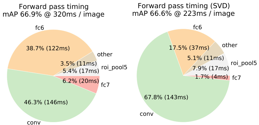
fc6 and fc7 take \(45\%\) of the time.Keeping the top 1024 singular values of the \(25088 \times 4096\) fc6 matrix and the top 256 of the \(4096 \times 4096\) fc7 matrix reduces runtime by more than \(30\%\) — 320 ms per image at \(66.9\%\) mAP becomes 223 ms at \(66.6\%\) — for a \(0.3\) point drop in mAP and without any further fine-tuning after compression.
Training and testing time
For VGG16, training falls from 84 hours to \(9.5\), a \(9\times\) reduction, and \(2.7\times\) against SPPnet’s 25 hours. Test rate falls from \(47.0\) s per image to \(0.32\) s, a factor of \(146\), or \(213\) with truncated SVD at \(0.22\) s. SPPnet, using its five scales, runs at \(2.3\) s per image. Hundreds of gigabytes of disk storage are eliminated because nothing is cached.
Which layers to fine-tune
For the less deep networks of the SPPnet paper, fine-tuning only the fully connected layers appeared sufficient. It is not sufficient for very deep networks. Freezing all thirteen VGG16 convolutional layers, so that only the fully connected layers learn, decreases mAP from \(66.9\%\) to \(61.4\%\) — an ablation that emulates single-scale SPPnet training, and the direct verification that training through the RoI pooling layer matters. Not all convolutional layers need updating either. conv1 is generic and task independent, and allowing it to learn has no meaningful effect. For VGG16 it is necessary to update layers from conv3_1 and up, 9 of the 13 convolutional layers: learning from conv2_1 gains only \(+0.3\) points and slows training by \(1.3\times\) (12.5 hours against \(9.5\)), and updating from conv1_1 over-runs GPU memory.
Sparse proposals as a cascade
Classifying a sparse set of proposals is a form of cascade in which the proposal mechanism first rejects a vast number of candidates, leaving the classifier a small set to evaluate. If proposals served a purely computational role, adding more of them should not harm mAP.
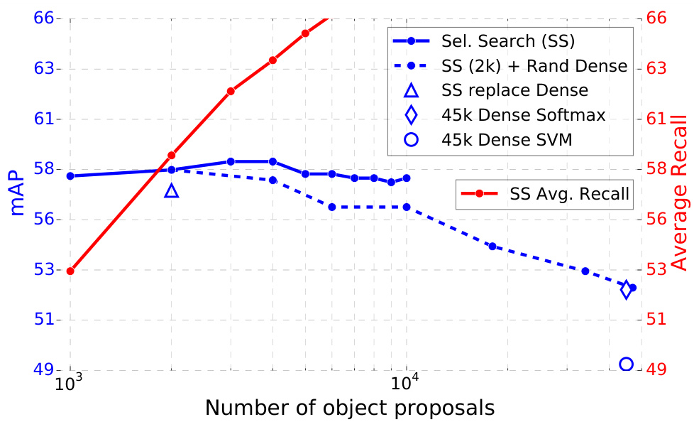
Sweeping selective search from 1k to 10k proposals per image, retraining and retesting model M each time, mAP rises and then falls slightly. Swamping the deep classifier with more proposals does not help and slightly hurts. Densely generated boxes, at about 45k per image over scale, position and aspect ratio, do worse still: replacing each selective search box by its closest dense box costs 1 point, adding growing numbers of dense boxes to the 2k sparse ones drives mAP down to \(53.0\%\), and training and testing on 45k dense boxes alone gives \(52.9\%\). Dense boxes with SVMs and hard negative mining are worse again at \(49.3\%\). Average Recall, the standard proxy for proposal quality, does not correlate with mAP once the number of proposals per image is varied, so it must be used with care.
Everything in the detector is now learned end to end except the proposals, and selective search on the CPU is now the dominant cost of a detection.
NoteOutcomes and concepts
Learning outcomes
- roi-pooling-shared-computation Explain how RoI pooling lets all proposals share one convolutional forward pass.
- compare-detector-generations Compare R-CNN, Fast R-CNN and Faster R-CNN on accuracy and speed, and name the bottleneck each removed.
Concepts
- truncated-svd factorising a \(u \times v\) fully connected weight matrix at rank \(t\) cuts its parameters to \(t(u+v)\) and detection time by more than \(30\%\), for a \(0.3\) mAP drop
- roi-pooling fine-tuning the convolutional layers through it is worth \(5.5\) mAP on VGG16, and
conv3_1and up is the range that pays
Faster R-CNN: region proposal networks and anchors
Ren et al., “Faster R-CNN: Towards Real-Time Object Detection with Region Proposal Networks”, observe that selective search takes about 2 seconds per image on a CPU implementation, an order of magnitude slower than the detection network it feeds, and that EdgeBoxes, at \(0.2\) s per image, still consumes as much running time as detection. Reimplementing a proposal algorithm on the GPU would ignore the down-stream network and miss the opportunity to share computation. The change made instead is algorithmic: the proposals are computed by a network over the same features.
A Region Proposal Network takes an image of any size and outputs a set of rectangular object proposals, each with an objectness score, where objectness measures membership to a set of object classes against background. It is a fully convolutional network sharing a common set of convolutional layers with the detector — five shareable layers in the Zeiler and Fergus model, thirteen in VGG-16.
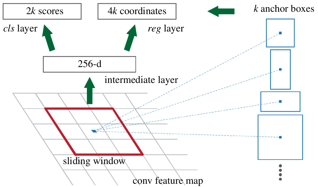
cls and reg layers. Right: detections from RPN proposals on PASCAL VOC 2007 across a wide range of scales and aspect ratios.A small network is slid over the convolutional feature map output by the last shared layer. It takes as input an \(n \times n\) spatial window of that map, with \(n = 3\), and maps it to a lower-dimensional feature — 256-d for ZF, 512-d for VGG, followed by ReLU. That feature goes into two sibling fully connected layers: a box-regression layer reg and a box-classification layer cls. Because the mini-network operates in a sliding-window fashion, its fully connected layers are shared across all spatial locations, and the architecture is naturally implemented as an \(n \times n\) convolutional layer followed by two sibling \(1 \times 1\) convolutional layers. The effective receptive field on the input image is large: 171 pixels for ZF and 228 for VGG.
Anchors
At each sliding-window location \(k\) region proposals are predicted simultaneously, so reg has \(4k\) outputs encoding the coordinates of \(k\) boxes and cls has \(2k\) scores estimating the probability of object and not-object for each proposal. The \(k\) proposals are parameterised relative to \(k\) reference boxes, the anchors. An anchor is centred at the sliding window in question and is associated with a scale and an aspect ratio; by default three scales with box areas \(128^2\), \(256^2\) and \(512^2\) pixels and three aspect ratios \(1{:}1\), \(1{:}2\) and \(2{:}1\) are used, yielding \(k = 9\) anchors at each position. For a feature map of size \(W \times H\), typically about 2400 positions, there are \(WHk\) anchors in total.
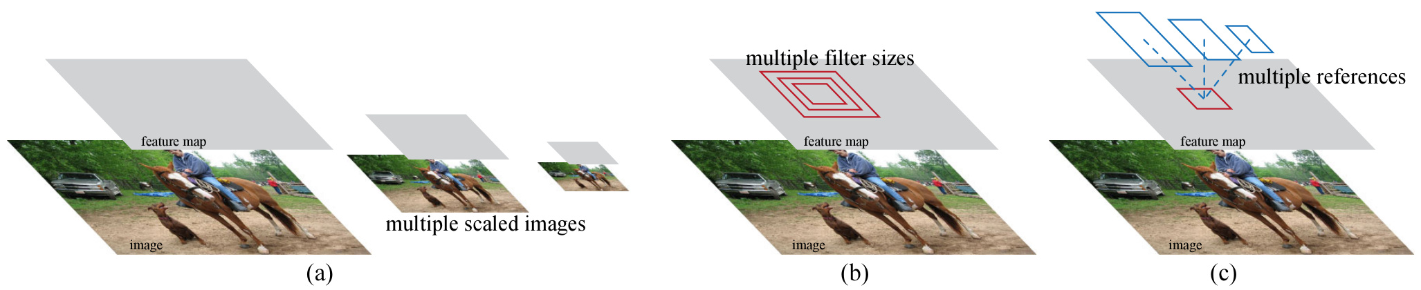
The two established approaches to multiple scales are an image or feature pyramid, useful but time-consuming, and a pyramid of filters, in which models of different aspect ratios are trained separately with different filter sizes such as \(5 \times 7\) and \(7 \times 5\). The anchor scheme is a pyramid of regression references: images, feature maps and filters are all of a single scale, and the multi-scale behaviour comes from regressing with reference to boxes of multiple scales and aspect ratios. That is what lets the single-scale features be shared with the detector at no extra cost for scale.
Anchors are also translation invariant, in both the anchors themselves and the functions that compute proposals relative to them: if an object is translated, the proposal translates and the same function predicts it at the new location. The property also reduces model size. For \(k = 9\) anchors the output layer is a \((4+2) \times 9\)-dimensional convolutional layer with \(2.8 \times 10^4\) parameters against MultiBox’s \((4+1) \times 800\)-dimensional fully connected output layer with \(6.1 \times 10^6\); MultiBox generates its 800 anchors by \(k\)-means and is not translation invariant.
The RPN loss
A binary class label of being an object or not is assigned to each anchor by two rules.
A positive label goes to the anchor or anchors with the highest IoU overlap with a ground-truth box, or to any anchor with IoU higher than \(0.7\) with any ground-truth box.
The second condition usually suffices, but the first is retained because in rare cases it finds no positive sample. A single ground-truth box may make several anchors positive.
A negative label goes to a non-positive anchor whose IoU is lower than \(0.3\) for all ground-truth boxes. Anchors that are neither positive nor negative do not contribute to the training objective.
With these definitions the objective for an image follows the multi-task loss of Fast R-CNN:
\[L(\{p_i\}, \{t_i\}) = \frac{1}{N_{cls}} \sum_i L_{cls}(p_i, p_i^*) + \lambda \frac{1}{N_{reg}} \sum_i p_i^* L_{reg}(t_i, t_i^*).\]
Here \(i\) indexes an anchor in the mini-batch, \(p_i\) is the predicted probability that anchor \(i\) is an object, and \(p_i^*\) is 1 if the anchor is positive and 0 if negative. \(L_{cls}\) is log loss over the two classes. For regression, \(t_i\) is the vector of four parameterised coordinates of the predicted box and \(t_i^*\) that of the ground-truth box associated with a positive anchor, and \(L_{reg}(t_i, t_i^*) = R(t_i - t_i^*)\) with \(R\) the smooth \(L_1\) loss defined in Fast R-CNN. The factor \(p_i^*\) means the regression loss is active only for positive anchors. The two terms are normalised by \(N_{cls}\), the mini-batch size of 256, and \(N_{reg}\), the number of anchor locations, about 2400, and weighted by \(\lambda = 10\) so that both contribute roughly equally. The result is insensitive to \(\lambda\) over a wide range: mAP moves from \(69.9\%\) at \(\lambda = 10\) to \(68.9\%\) at \(1\) and \(69.1\%\) at \(100\).
The coordinates are parameterised as before, now relative to an anchor \(a\) rather than a proposal:
\[t_\mathrm{x} = (x - x_a)/w_a, \quad t_\mathrm{y} = (y - y_a)/h_a, \quad t_\mathrm{w} = \log(w/w_a), \quad t_\mathrm{h} = \log(h/h_a),\]
with \(t^*\) defined identically from the ground-truth box. One difference from RoI-based regression matters. There, boxes are regressed from features pooled from arbitrarily sized RoIs and one set of regression weights serves all region sizes. Here every prediction is made from features of the same spatial size, \(3 \times 3\), so \(k\) separate regressors are learned, one per scale and aspect ratio, and they do not share weights. Boxes of varying size remain predictable because of the anchor design, not because the features vary.
Predictions may exceed the receptive field. The learned average proposal for the \(512^2\), \(1{:}2\) anchor with the ZF net is \(355 \times 715\) pixels, larger than the 171-pixel receptive field. Such a prediction is not impossible — the extent of an object can be inferred roughly when only its middle is visible.
NoteOutcomes and concepts
Learning outcomes
- rpn-and-anchors Design a Region Proposal Network with translation-invariant anchor boxes.
Concepts
- region-proposal-network a \(3 \times 3\) window slid over the last shared feature map, projected to 256-d or 512-d and fed to sibling \(1 \times 1\)
clsandreglayers, emits \(2k\) objectness scores and \(4k\) coordinates per location - anchors \(k = 9\) reference boxes of three scales and three aspect ratios per location form a pyramid of regression references, translation invariant and needing only \(2.8 \times 10^4\) output parameters
- multi-task-rpn-loss objectness log loss plus smooth \(L_1\) box loss, normalised by \(N_{cls} = 256\) and \(N_{reg} \approx 2400\) and balanced by \(\lambda = 10\)
- faster-r-cnn the proposal stage becomes a network over the features the detector already computes, so its marginal cost is about 10 ms per image
Sharing features between the RPN and the detector
What is shared is one object: the convolutional feature map computed once from the whole image. The RPN and the detector are two heads reading that same map, and everything upstream of it belongs to neither of them.
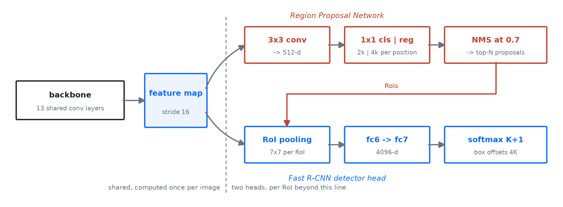
The dashed line is the answer to “where”: every layer left of it runs once on the image, and every layer right of it runs once per RoI. Sharing is what makes the proposal step cost 10 ms rather than the 1510 ms selective search spends, because the RPN’s own layers are a \(3 \times 3\) convolution and two \(1 \times 1\) convolutions on a map the detector needed anyway.
The RPN is trained end to end by back-propagation and SGD, following the image-centric sampling strategy of Fast R-CNN. Each mini-batch arises from a single image that contains many positive and negative anchors. Optimising over all anchors in the image would bias the objective towards negatives, since they dominate, so 256 anchors are sampled at random from one image with a positive-to-negative ratio of up to \(1{:}1\); if an image has fewer than 128 positive samples, the mini-batch is padded with negatives. New layers are initialised from a zero-mean Gaussian with standard deviation \(0.01\) and all other layers from an ImageNet classification model. On PASCAL VOC the learning rate is \(0.001\) for 60k mini-batches and \(0.0001\) for the next 20k, with momentum \(0.9\) and weight decay \(0.0005\).
Implementation details that matter
- Images are re-scaled so that the shorter side is \(s = 600\) pixels. The total stride on the last convolutional layer is 16 pixels for both ZF and VGG, which is about 10 pixels on a typical PASCAL image of roughly \(500 \times 375\) before resizing. Even so large a stride gives good results.
- Anchors crossing the image boundary are ignored during training. For a typical \(1000 \times 600\) image there are roughly 20000 anchors, about \(60 \times 40 \times 9\); ignoring cross-boundary ones leaves about 6000. Kept in, they introduce large error terms that are difficult to correct and training does not converge. At test time the fully convolutional RPN is applied to the whole image and cross-boundary proposals are clipped to the boundary.
- Proposals overlap heavily, so non-maximum suppression is applied to them on the basis of their
clsscores, with the IoU threshold fixed at \(0.7\), leaving about 2000 proposal regions per image. The top-\(N\) ranked proposals are then used for detection. This does not harm detection accuracy.
What sharing buys
Timings on a K40 GPU make the case plainly. Selective search plus Fast R-CNN with VGG-16 spends 146 ms on convolutions, 1510 ms on proposals and 174 ms region-wise, for 1830 ms in total — \(0.5\) fps. With the RPN sharing features, the proposal step costs 10 ms and the region-wise computation falls to 47 ms because there are fewer proposals, for 198 ms in total, or 5 fps. With the ZF net the figures are 31, 3 and 25 ms, 59 ms in total, or 17 fps.
Accuracy improves at the same time. On VOC 2007 with the ZF net, selective search with 2000 proposals gives \(58.7\%\) mAP and EdgeBoxes with 2000 gives \(58.6\%\), while the shared RPN with up to 300 proposals gives \(59.9\%\). Stopping after step 2 of the alternating recipe, so that the networks do not share, reduces this to \(58.7\%\): the third step, in which detector-tuned features are used to fine-tune the RPN, improves proposal quality. With VGG-16 the unshared variant gives \(68.5\%\) and the shared one \(69.9\%\), both above the \(66.9\%\) selective search baseline, and training on the union of VOC 2007 trainval and VOC 2012 trainval raises it to \(73.2\%\).
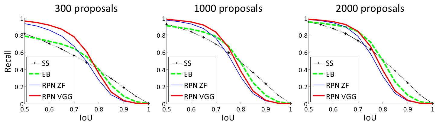
The ablations separate the contributions of the two RPN outputs. Removing the cls layer at test time, so that \(N\) proposals are sampled at random from the unscored regions, leaves mAP nearly unchanged at \(55.8\%\) for \(N = 1000\) but degrades it to \(44.6\%\) for \(N = 100\): the objectness scores are what make a short proposal list accurate. Removing the reg layer, so that the proposals become the anchor boxes themselves, drops mAP to \(52.1\%\). Anchors of multiple sizes and ratios earn their place: one anchor per position gives \(65.8\%\) or \(66.7\%\) depending on its scale, three ratios at one scale give \(68.8\%\), three scales at one ratio give \(69.8\%\), and three scales with three ratios \(69.9\%\). Recall against IoU is only loosely related to detection accuracy and is better used to diagnose a proposal method than to evaluate one; what the curves show is that the RPN degrades gracefully as its proposal count falls from 2000 to 300, where selective search and EdgeBoxes lose recall faster.
NoteOutcomes and concepts
Learning outcomes
- feature-sharing-training Train an RPN and a Fast R-CNN detector so that they share one set of convolutional features.
- compare-detector-generations Compare R-CNN, Fast R-CNN and Faster R-CNN on accuracy and speed, and name the bottleneck each removed.
Concepts
- four-step-alternating-training four steps progressively tie the convolutional layers together, and the third step — re-tuning the RPN on detector-tuned features — is where the shared model gains \(1.2\) mAP over the unshared one
- faster-r-cnn one network runs at 198 ms per image with VGG-16 and 59 ms with ZF, against 1830 ms for selective search plus Fast R-CNN
- region-proposal-network proposal quality comes from
clsandregtogether: without scores a 100-proposal list collapses to \(44.6\%\) mAP, without regression the anchors alone give \(52.1\%\) - anchors cross-boundary anchors are dropped during training, leaving about 6000 of 20000, and proposals are reduced by non-maximum suppression at IoU \(0.7\)
Benchmarks and the two-stage cascade
Placed side by side on VOC 2007 test with VGG-16, the three generations read: R-CNN with bounding-box regression at \(66.0\%\) mAP and 47 s per image; Fast R-CNN at \(66.9\%\) and \(0.32\) s, or \(68.1\%\) when examples marked “difficult” in PASCAL are removed; Faster R-CNN at \(69.9\%\) with 300 shared-feature proposals and \(0.198\) s. On VOC 2012, Fast R-CNN reaches \(65.7\%\) and Faster R-CNN \(70.4\%\) trained on 07++12.
Deeper backbones convert directly into accuracy. On the COCO validation set, replacing VGG-16 by the 101-layer residual network raises Faster R-CNN from \(41.5\%/21.2\%\) to \(48.4\%/27.2\%\) in mAP@\(0.5\) and mAP@\([.5, .95]\). With further orthogonal improvements, He et al. obtained a single-model result of \(55.7\%/34.9\%\) and an ensemble of \(59.0\%/37.4\%\) on the COCO test-dev set, which took first place in the COCO 2015 detection competition; the same system won ILSVRC 2015 detection by \(8.5\%\) absolute over second place. The RPN learns to propose regions entirely from data, which is why it benefits from better features rather than being limited by a fixed grouping heuristic.
MS COCO
MS COCO has 80 object categories, with 80k training, 40k validation and 20k test-dev images, and its standard metric averages mAP over IoU thresholds in \([0.5 : 0.05 : 0.95]\). Two changes are made for it: a fourth anchor scale of \(64^2\) is added, mainly to handle small objects, and the negative samples in Fast R-CNN are defined as those with maximum IoU with ground truth in \([0, 0.5)\) rather than \([0.1, 0.5)\), so that the \([0, 0.1)\) samples are visited at all. On test-dev, Faster R-CNN with 300 proposals reaches \(42.7\%\) mAP@\(0.5\) and \(21.9\%\) mAP@\([.5, .95]\), against \(39.3\%\) and \(19.3\%\) for the paper’s own Fast R-CNN baseline with 2000 selective search boxes. The gain is \(2.2\) points on the stricter metric against \(2.8\) on the looser one, which indicates that the RPN improves localisation accuracy at high IoU thresholds.
More detection data keeps helping
Evaluating the COCO-trained model directly on PASCAL VOC 2007, with no fine-tuning on any VOC data — possible because the VOC categories are a subset of COCO’s — gives \(76.1\%\) mAP, already better than the \(73.2\%\) obtained by training on VOC 07+12. Fine-tuning the COCO model on VOC 07+12 reaches \(78.8\%\), an increase of \(5.6\) points from the extra data, with the best AP for every individual category; VOC 2012 reaches \(75.9\%\). Test-time speed is unchanged at about 200 ms per image.
Why two stages
The comparison against one-stage dense detection is run under matched conditions. The one-stage system is a Fast R-CNN in which the “proposals” are dense sliding windows of three scales (\(128\), \(256\), \(512\)) and three aspect ratios (\(1{:}1\), \(1{:}2\), \(2{:}1\)) — 20000 windows — and which predicts class-specific scores and regresses boxes from those windows. With the ZF model, the one-stage system reaches \(53.9\%\) mAP against \(58.7\%\) for the two-stage cascade of 300 unshared RPN proposals plus a detector, a gap of \(4.8\) points; evaluating the one-stage system over five scales, as its image-pyramid ancestor does, gives \(53.8\%\) and changes nothing.
ImportantThe stated reason for the gap
In the one-stage design the region-wise features come from a sliding window of one aspect ratio over a scale pyramid, and those same features must determine both the location and the category of an object. In the second stage of the cascade the region-wise features are adaptively pooled from proposal boxes that more faithfully cover the features of the regions. It is the adaptive pooling, not the window count, that the comparison isolates — the one-stage system is also slower, having far more proposals to process.
NoteOutcomes and concepts
Learning outcomes
- compare-detector-generations Compare R-CNN, Fast R-CNN and Faster R-CNN on accuracy and speed, and name the bottleneck each removed.
- rpn-and-anchors Design a Region Proposal Network with translation-invariant anchor boxes.
Concepts
- faster-r-cnn \(73.2\%\) mAP on VOC 2007 and \(42.7\%\) mAP@\(0.5\) on COCO test-dev with 300 proposals, rising to \(78.8\%\) with COCO pre-training and scaling directly with a 101-layer backbone
- anchors a fourth scale of \(64^2\) is added for COCO, where small objects are common, which is the anchor set’s only dataset-specific adjustment
The region-based family, consolidated
Three generations, three bottlenecks removed.
- R-CNN classifies about 2000 warped proposals independently, each with its own CNN forward pass, and trains in three stages with features cached to disk. Its bottleneck is per-proposal convolution.
- Fast R-CNN projects proposals onto a feature map computed once per image and pools them to a fixed size, then trains classification and localisation together in one stage. Its bottleneck is the externally computed proposals, at about 2 seconds per image on the CPU.
- Faster R-CNN computes the proposals with a small convolutional network over the same shared features, at a marginal cost of 10 ms, and trains it to share those features with the detector. Its remaining cost is the region-wise computation above RoI pooling — 47 ms of the 198 ms per image with VGG-16.
Three pieces of machinery recur throughout and are worth holding separately from the architectures that carry them: the scale-invariant, log-space box parameterisation \((t_x, t_y, t_w, t_h)\), unchanged from R-CNN’s appendix to the RPN loss; the multi-task objective that trains classification and localisation together; and IoU thresholds as the mechanism for turning a continuous overlap into training labels — \(0.5\) for fine-tuning positives, \(0.3\) for SVM negatives, \(0.7\) and \(0.3\) for anchors, \(0.6\) for regression pairs, and \(0.7\) for proposal suppression.
NoteOutcomes and concepts
Learning outcomes
- compare-detector-generations Compare R-CNN, Fast R-CNN and Faster R-CNN on accuracy and speed, and name the bottleneck each removed.
- detection-task-and-evaluation State the object detection problem and evaluate a detector with IoU-based mean average precision.
- multi-task-loss-and-single-stage-training Train a detector in one stage with a multi-task classification and localisation loss.
- feature-sharing-training Train an RPN and a Fast R-CNN detector so that they share one set of convolutional features.
Key ideas, and what follows
Key ideas
Applying a high-capacity CNN to bottom-up region proposals broke a plateau: \(53.7\%\) mAP on VOC 2010 against \(33.4\%\) for DPM v5, and \(31.4\%\) against \(24.3\%\) on ILSVRC2013.
Localisation as regression reached \(30.5\%\) on VOC 2007 and sliding windows were obstructed by \(195 \times 195\) receptive fields at stride 32. Regions sidestep both.
Supervised pre-training on ILSVRC followed by domain-specific fine-tuning on warped proposals is worth 8.0 mAP points, concentrated in the fully connected layers.
The convolutional features transfer nearly intact, which is what makes detection possible on a dataset far smaller than ImageNet.
Error analysis showed that poor localisation, not background confusion, dominated R-CNN’s false positives, and a linear ridge regression on \(\text{pool}_5\) features recovered 3 to 4 mAP.
Measuring the error distribution before adding machinery is the method, not the result.
RoI pooling with hierarchical mini-batch sampling makes the convolutional work independent of the proposal count: \(9\times\) faster training and \(213\times\) faster testing than R-CNN, with no feature cache.
A mini-batch of \(N = 2\) images and 64 RoIs each is roughly \(64\times\) cheaper than 128 RoIs from 128 images, because RoIs from one image share its passes.
Back-propagating through RoI pooling to fine-tune the convolutional layers is what deep backbones need: freezing VGG16’s thirteen conv layers costs \(5.5\) mAP, \(66.9\%\) falling to \(61.4\%\).
This is the capability SPPnet lacked, and the reason its accuracy was capped on very deep networks.
One multi-task loss replaces three training stages, and the softmax it trains slightly outperforms post-hoc SVMs.
Multi-task training also improves pure classification by \(0.8\) to \(1.1\) mAP, so the joint objective is not merely a convenience.
Sparse proposals act as a cascade rather than as an approximation to dense boxes: mAP rises then falls with proposal count, and 45k dense boxes give \(52.9\%\) against \(57.7\%\) for sparse ones.
Average Recall does not track mAP once the proposal count varies, so it diagnoses a proposal method rather than evaluating it.
Anchors — \(k = 9\) reference boxes of three scales and three aspect ratios — replace image and filter pyramids, are translation invariant, and need \(2.8 \times 10^4\) output parameters against MultiBox’s \(6.1 \times 10^6\).
Multi-scale prediction from a single-scale feature map is what lets the proposal stage share the detector’s features.
Sharing convolutions makes proposal generation nearly free: 10 ms per image, and 5 fps end to end with VGG-16 against \(0.5\) fps for selective search plus Fast R-CNN.
300 learned proposals also beat 2000 selective search boxes, so sharing improves accuracy as well as speed.
Under matched conditions the two-stage cascade beats one-stage dense detection, \(58.7\%\) against \(53.9\%\) mAP with the ZF model.
The second stage pools features adaptively from boxes that cover the region, where a one-stage detector must decide from a generic sliding window.
The next unit, Fast Object Detection Networks, keeps the anchors and the box regression and removes the second stage. YOLO predicts all boxes and class probabilities from an \(S \times S\) grid in one forward pass; SSD tiles default boxes over feature maps of several resolutions and runs small convolutional predictors on each; YOLOv2 restores anchors, choosing them by \(k\)-means over the training boxes rather than by hand. The \(4.8\)-point result above is the claim those detectors contest, and knowing which quantities that comparison held fixed is what makes their evidence readable. Feature Pyramid Networks then return to this architecture, attaching an RPN and a Fast R-CNN head to each level of a top-down pyramid so that every level handles a narrow range of scales.
References
Girshick, Ross, et al. “Rich feature hierarchies for accurate object detection and semantic segmentation.” Proceedings of the IEEE conference on computer vision and pattern recognition. 2014.
Girshick, Ross. “Fast r-cnn.” Proceedings of the IEEE international conference on computer vision. 2015.
Ren, S., He, K., Girshick, R., & Sun, J. (2015). Faster r-cnn: Towards real-time object detection with region proposal networks. Advances in neural information processing systems, 28.