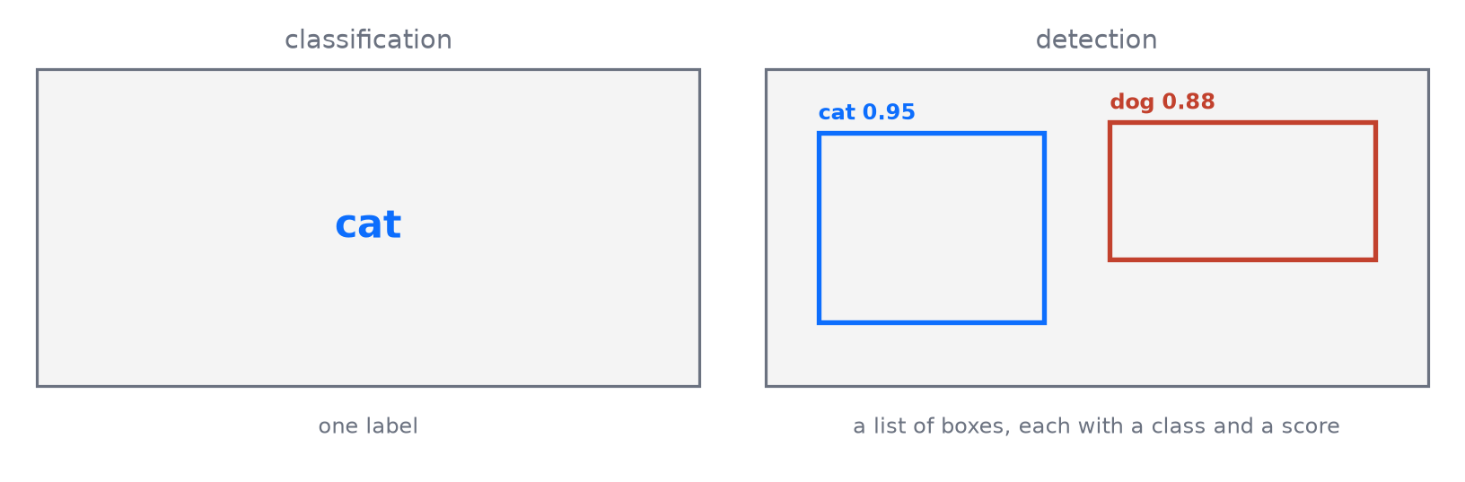
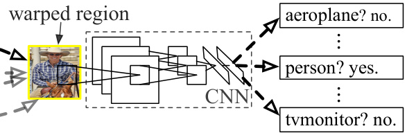
Three modules
A region proposal generator, independent of category
A large convolutional network , one fixed-length vector per region
A set of class-specific linear SVMs
Detection recast as region classification — recognition using regions .
Trial and error, by proposal
Selective search in fast mode emits about 2000 candidate boxes per imageThe method is agnostic to the algorithm — objectness, CPMC and MCG are alternatives
The generator is a black box: nothing in it is learned
Every proposal is a guess to be scored, and almost all of them are wrong.
Warping to a fixed size
Proposals warped to \(227 \times 227\) .
The network requires a fixed \(227 \times 227\) input; proposals are arbitrary rectangles
Anisotropic warping with context padding : dilate the box so \(p = 16\) pixels of context survive, then warpBeats square crops by 3 to 5 mAP points
One forward pass per proposal, 2000 per image, each giving a 4096-d vector.
The aspect ratio is destroyed by the warp. Where the source rectangle extends past the image, the missing data is replaced with the image mean. Appendix A compares this against the tightest square with and without context.
Scoring the candidates
Each 4096-d vector is scored by the linear SVM of each class
\(N + 1\) classes: \(N\) object types and one background classClass-specific work is one matrix product, \(2000 \times 4096\) against \(4096 \times N\)
CNN parameters are shared across categories, so the 13 s per image is amortised over every class.
Non-maximum suppression
For one class, with \(\mathcal{B} = \{(b_i, s_i)\}\) the scored boxes and threshold \(\tau\) :
\[
\begin{aligned}
m &\leftarrow \operatorname*{argmax}_{i \,:\, (b_i, s_i) \in \mathcal{B}} s_i,\\
\mathcal{D} &\leftarrow \mathcal{D} \cup \{b_m\},\\
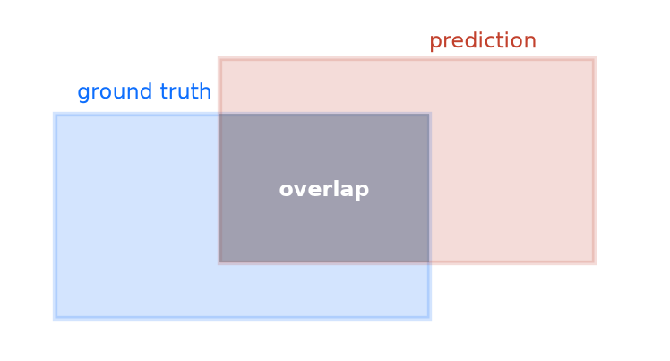
\mathcal{B} &\leftarrow \mathcal{B} \setminus \big(\{(b_m, s_m)\} \cup \{i : \mathrm{IoU}(b_m, b_i) > \tau\}\big)
\end{aligned}
\]
Repeated until \(\mathcal{B}\) is empty, from \(\mathcal{D} = \emptyset\) , independently per class.
The same procedure, as pseudocode
Greedy: a box once kept is never reconsidered
Run per class , so boxes of different classes never suppress each other
Boxes that survive are still off target
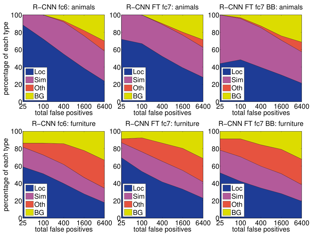
Loc — IoU with the correct class between \(0.1\) and \(0.5\) , or a duplicateSignificantly more errors are Loc than background or wrong-class
The reverse of the pattern DPM shows
The features discriminate; the boundaries are loose.
Bounding-box regression
A surviving proposal \(P = (P_x, P_y, P_w, P_h)\) and its \(\text{pool}_5\) feature give:
\[(d_x, d_y, d_w, d_h) = \mathbf{W}\,\boldsymbol{\phi}_5(P), \qquad \mathbf{W} \in \mathbb{R}^{4 \times 4096}\]
applied as a scale-invariant shift and a log-space rescaling:
\[
\begin{aligned}
\hat{G}_x &= P_w d_x + P_x, & \hat{G}_w &= P_w e^{d_w},\\
\hat{G}_y &= P_h d_y + P_y, & \hat{G}_h &= P_h e^{d_h}
\end{aligned}
\]
Worth 3 to 4 mAP: \(54.2\%\) to \(58.5\%\) on VOC 2007.
Fitting the regressor
The targets
\[
\begin{aligned}
t_x &= (G_x - P_x)/P_w\\
t_y &= (G_y - P_y)/P_h\\
t_w &= \log(G_w/P_w)\\
t_h &= \log(G_h/P_h)
\end{aligned}
\]
Ridge regression, \(\lambda = 1000\) .
Fitted once per class
A proposal is used only if its IoU with the assigned ground truth exceeds \(0.6\)
Transforming a distant \(P\) into \(G\) is not well posed
At test time the transform is applied once to each scored proposal. Iterating it — re-scoring the predicted box and predicting again — was tried and does not improve results.
Training, in three stages
Pre-train the CNN on ILSVRC2012 image-level labelsFine-tune it on warped proposals, with a fresh \((N+1)\) -way layer, at one tenth the learning rateFit the SVMs , then the regressors , on cached features
Two definitions of a positive: IoU \(\ge 0.5\) for fine-tuning, ground-truth boxes only for the SVMs.
Fine-tuning has too little data, and the relaxed definition supplies roughly 30 times as many positives in the form of jittered windows. SVM training does not need the extra data, so it uses exact positives with hard negative mining. Applying the fine-tuned softmax directly as the detector drops VOC 2007 from 54.2% to 50.9%.
What it cost
The bottlenecks
A full forward pass per proposal , thousands per image
Features written to disk between stages
Three separate training stages
The numbers, VGG16
\(2.5\) GPU-days to extract features for VOC07 trainvalHundreds of gigabytes of storage
\(47\) s per image at test time
Nothing is shared between two proposals overlapping by 90%.
Fast R-CNN and the RoI pooling layer
One pass over the image
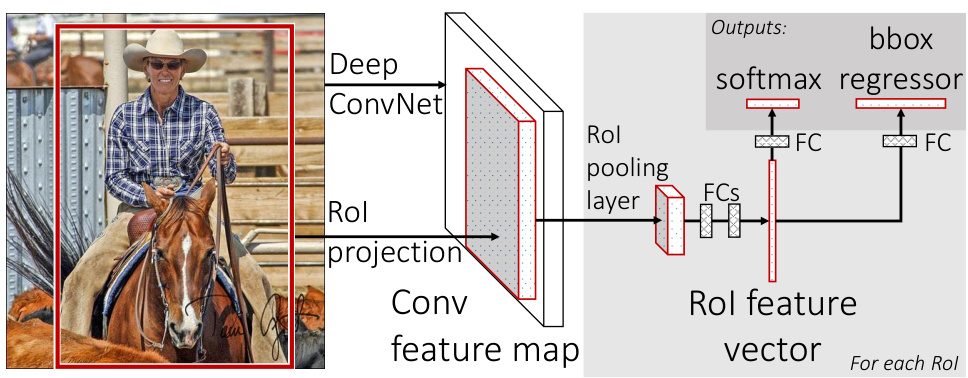
The whole image through the convolutional layers once; each RoI pooled from the shared map, then two sibling outputs — softmax over \(K+1\) classes, and per-class box offsets.
What an RoI is
An RoI is a rectangular window on the conv feature map,
\[(r, c, h, w)\]
its top-left corner, height and width.
One RoI is one proposal, projected onto the map by dividing by the total stride
A \(320 \times 480\) proposal becomes about \(20 \times 30\) positions at stride 16
The proposals still come from selective search. Only the forward pass is shared.
What RoI pooling computes
The \(h \times w\) window is divided into an \(H \times W\) grid, the \((i,j)\) -th cell covering
\[
\mathcal{R}_{ij} = \left\{ (y, x) \;:\;
\begin{aligned}
r + \left\lfloor \tfrac{(i-1)h}{H} \right\rfloor &\le y < r + \left\lceil \tfrac{ih}{H} \right\rceil\\
c + \left\lfloor \tfrac{(j-1)w}{W} \right\rfloor &\le x < c + \left\lceil \tfrac{jw}{W} \right\rceil
\end{aligned}
\right\}
\]
\[\mathbf{Y}_{k,i,j} = \max_{(y,x) \in \mathcal{R}_{ij}} \mathbf{X}_{k,y,x}, \qquad \mathbf{Y} \in \mathbb{R}^{C \times H \times W}\]
Any RoI, whatever its size, yields the same fixed shape — which is what the fully connected layers require.
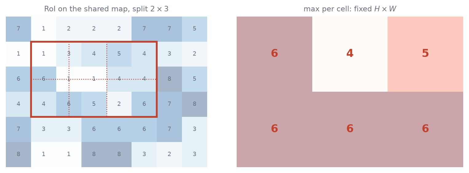
The grid, drawn
Pooling is per channel, and the output size does not depend on the RoI.
Backward, the layer routes each gradient to whichever input position attained the maximum, accumulating over every RoI that selected it. That is the step SPPnet lacked, and it is why the convolutional layers below can be fine-tuned at all — freezing VGG16’s thirteen conv layers costs 5.5 mAP.
One multi-task loss
\[L(p, u, t^u, v) = L_{\mathrm{cls}}(p, u) + \lambda\,[u \ge 1]\,L_{\mathrm{loc}}(t^u, v)\]
\(L_{\mathrm{cls}}(p, u) = -\log p_u\) , log loss over the \(K+1\) softmax outputs\([u \ge 1]\) is zero for background, \(u = 0\) , which has no ground-truth box\(L_{\mathrm{loc}}\) sums \(\mathrm{smooth}_{L_1}\) over \((t_x, t_y, t_w, t_h)\) , with \(\lambda = 1\)
Three training stages collapse into one, and the softmax it trains outperforms post-hoc SVMs.
Smooth \(L_1\)
\[\mathrm{smooth}_{L_1}(x) = \begin{cases} 0.5x^2 & |x| < 1\\ |x| - 0.5 & \text{else}\end{cases}\]
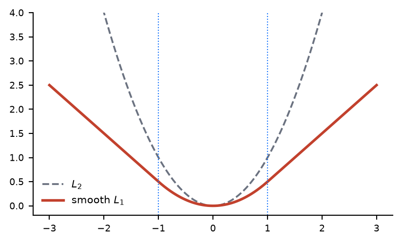
Quadratic near zero, linear beyond
\(L_2\) with unbounded targets needs careful learning-rate tuning to avoid exploding gradients
What RoI pooling bought
Speed
\(47\) s per image falls to \(0.32\) sTraining \(9\times\) faster
The disk cache disappears
What remains
Proposals still come from selective search , about 2 s per image on CPU
Low-quality candidates, thousands of them
The convolutional work no longer grows with the proposal count. The proposal step now dominates.
Faster R-CNN and the region proposal network
Proposals from the same features
Selective search costs about 2 s per image, an order of magnitude slower than the detector it feeds
EdgeBoxes at \(0.2\) s still consumes as much time as detection
A GPU reimplementation would ignore the network and miss the chance to share
The change is algorithmic: compute the proposals with a network over the features already there.
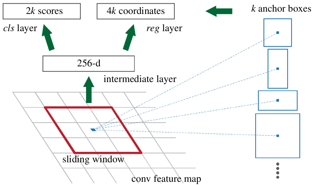
The sliding window on the feature map
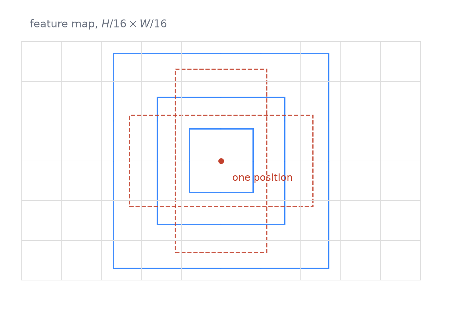
A VGG backbone at stride 16 maps an image to \(H/16 \times W/16\) positions
An \(n \times n\) window, \(n = 3\) , maps each position to 512-d
Then two sibling \(1 \times 1\) convolutions, cls and reg
Shared across all positions, so the head is three convolutions and nothing else.
Anchors
\(k = 9\) anchors per position: three scales \(128^2, 256^2, 512^2\) and three ratios \(1{:}1, 1{:}2, 2{:}1\) .
What each position predicts
cls, \(2k\) outputs
Object against background, for each anchor. The class is not decided here.
reg, \(4k\) outputs
\[t_x = \frac{x - x_a}{w_a}, \;\; t_w = \log\frac{w}{w_a}\]
and likewise for \(y\) and \(h\) , relative to anchor \(a\) .
A pyramid of regression references , replacing pyramids of images or of filters.
Anchors are translation invariant: translate the object and the proposal translates, predicted by the same function. The output layer needs 2.8e4 parameters against MultiBox’s 6.1e6. Unlike RoI-based regression, the k regressors do not share weights, because every prediction is made from features of the same 3x3 spatial size.
The RPN loss
\[
\begin{aligned}
L(\{p_i\}, \{t_i\}) = \;& \frac{1}{N_{cls}} \sum_i L_{cls}(p_i, p_i^*)\\
+\;& \lambda \frac{1}{N_{reg}} \sum_i p_i^* L_{reg}(t_i, t_i^*)
\end{aligned}
\]
\(p_i^* = 1\) above IoU \(0.7\) , \(0\) below \(0.3\) , between contributes nothing\(N_{cls} = 256\) , \(N_{reg} \approx 2400\) , \(\lambda = 10\)
\(p_i^*\) makes the box loss active only on positive anchors.
Where the features are shared
Shared
The backbone and the feature map it produces, computed once per image .
Per RoI
The RPN head, and the detector head above RoI pooling — and the RPN’s surviving proposals are the detector’s RoIs.
4-step alternating training ties them: RPN, detector, RPN with shared layers fixed, detector head.
Trained independently the two would modify the shared layers in different ways. Approximate joint training merges them in one network and ignores the derivative with respect to the proposal coordinates; it gives close results at 25 to 50% less training time. Further iterations of the alternation produced negligible improvement.
What sharing buys
Selective search + Fast R-CNN
1510 ms
1830 ms
\(0.5\) fps
RPN, shared, VGG-16
10 ms
198 ms
5 fps
RPN, shared, ZF
3 ms
59 ms
17 fps
300 learned proposals also beat 2000 selective search boxes: \(59.9\%\) against \(58.7\%\) mAP.