Lecture notes — Fast Object Detection Networks
ver. 1.1.0, fast_object_detection_networks
← Fast Object Detection Networks
ver. 1.1.0 · 2026-09-02 08:25:08
Where this fits
The region-based family ends with Faster R-CNN: a shared backbone, a learned Region Proposal Network, RoI pooling, and a multi-task loss over classification and box regression. Proposals are almost free there, but the second stage is not — a small network still runs once per region, and the fastest reported configuration reaches about 7 frames per second.
The detectors in this unit remove the second stage. A single convolutional network is evaluated once and emits every box in the image, at 45 to 155 frames per second. Two questions follow from that decision, and the four sources answer them in turn: what does the prediction surface look like once there are no proposals, and what accuracy is lost when a detector stops looking twice.
Four sources are used throughout: Redmon, Divvala, Girshick and Farhadi (2016) on YOLO; Liu et al. (2016) on SSD; Redmon and Farhadi (2017) on YOLOv2 and YOLO9000; and Lin et al. (2017) on Feature Pyramid Networks.
Learning outcomes
single-shot-formulation— Formulate detection as one regression from image pixels to boxes and class probabilities over a fixed grid.yolo-loss-and-training— Train a grid detector with YOLO’s weighted sum-squared loss.yolo-error-profile— Diagnose a single-shot detector’s error profile and its structural limits.ssd-multiscale-default-boxes— Design a detector that predicts from default boxes tiled over feature maps of several resolutions.training-single-shot-detectors— Stabilise single-shot training with hard negative mining and aggressive augmentation.yolov2-design-improvements— Explain each YOLOv2 change and the mAP it contributes.joint-training-large-vocabulary— Combine detection and classification data over a label hierarchy to detect thousands of classes.feature-pyramid-construction— Build an in-network feature pyramid with a top-down pathway and lateral connections.fpn-in-a-detector— Attach an RPN and a Fast R-CNN head to a feature pyramid, and read the ablations that justify it.detector-design-tradeoffs— Choose a detector for a deployment constraint by reasoning about speed, accuracy and object scale.
Concepts introduced
- Unified object detection — the whole detection pipeline expressed as one network evaluated once per image, optimised directly on detection performance.
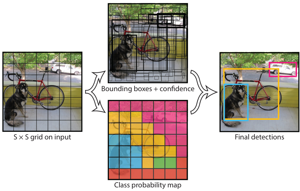
- Grid-based prediction — the image is divided into an \(S \times S\) grid, and the cell containing an object’s centre is responsible for predicting it.
- Multi-part detection loss — a sum-squared error loss whose coordinate, confidence and classification terms carry separate weights.
- Default boxes — reference boxes of several scales and aspect ratios tiled convolutionally over a feature map, the target of every offset prediction.
- Multi-scale feature maps for detection — predictions taken from several feature maps of decreasing resolution, so that scale is handled by choice of map.
- Hard negative mining — negative boxes sorted by confidence loss, with only the worst retained at a fixed ratio to the positives.
- Zoom-out augmentation — the training image placed on an enlarged mean-filled canvas, which synthesises small objects.
- Dimension clusters — anchor priors obtained by \(k\)-means over the training boxes under an IoU-based distance.
- Direct location prediction — box centres constrained to their own cell by a logistic activation on the predicted offset.
- Darknet-19 — a 19-layer convolutional backbone requiring 5.58 billion operations per image.
- WordTree — a tree of visual concepts built from WordNet, over which class probability is a product of conditionals along a path.
- Joint classification and detection training — detection images backpropagate the full loss; classification images backpropagate only the classification loss.
- Feature pyramid network — an in-network pyramid whose every level carries both fine resolution and strong semantics.
- Scale-based RoI assignment — an RoI routed to a pyramid level by the logarithm of its size.
YOLO’s unified detection
Unified object detection replaces the proposal-classify-rescore pipeline with a single convolutional network evaluated once per image. Redmon, Divvala, Girshick and Farhadi (2016) state the case against the alternative directly: those pipelines “are slow and hard to optimize because each individual component must be trained separately.”
Grid-based prediction is the shape given to the output. The image is divided into an \(S \times S\) grid. If the centre of an object falls into a grid cell, that cell is responsible for detecting that object. Each cell predicts \(B\) bounding boxes, and each box carries five numbers — \(x\), \(y\), \(w\), \(h\) and a confidence. The parameterisation matters:
The \((x, y)\) coordinates are the centre of the box relative to the bounds of the grid cell, and so lie between 0 and 1.
Width and height are predicted relative to the whole image, not to the cell, and are also normalised to \([0, 1]\).
Confidence is defined as \(\Pr(\text{Object}) \times \mathrm{IOU}^{\text{truth}}_{\text{pred}}\).
If no object exists in the cell the confidence should be zero; otherwise the target is the intersection over union between the predicted box and the ground truth. Confidence is therefore a prediction about the network’s own localisation quality, not only about presence.
Each cell additionally predicts \(C\) conditional class probabilities \(\Pr(\text{Class}_i \mid \text{Object})\). These are conditioned on the cell containing an object, and only one set is predicted per cell regardless of \(B\). The easy misreading is that the \(B\) boxes each carry a class; they do not. At test time the two quantities are multiplied,
\[\Pr(\text{Class}_i \mid \text{Object}) \times \Pr(\text{Object}) \times \mathrm{IOU}^{\text{truth}}_{\text{pred}} = \Pr(\text{Class}_i) \times \mathrm{IOU}^{\text{truth}}_{\text{pred}},\]
giving a class-specific confidence score for each box, which encodes both the probability of the class appearing in the box and how well the box fits the object. The predictions are encoded as an \(S \times S \times (B \times 5 + C)\) tensor. On PASCAL VOC the paper uses \(S = 7\), \(B = 2\) and \(C = 20\), so the final prediction is a \(7 \times 7 \times 30\) tensor.
The network has 24 convolutional layers followed by 2 fully connected layers. It is inspired by GoogLeNet, but in place of the inception modules it uses alternating \(1 \times 1\) reduction layers followed by \(3 \times 3\) convolutional layers. The convolutional layers extract features; the fully connected layers predict the output probabilities and coordinates.
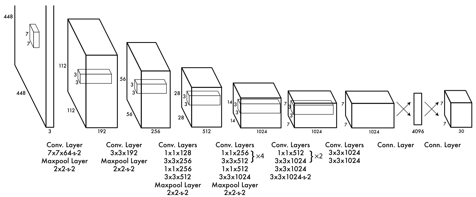
Fast YOLO is a smaller network of 9 convolutional layers instead of 24, with fewer filters in those layers. Other than the size of the network, all training and testing parameters are the same between YOLO and Fast YOLO.
Two properties separate this from the systems it replaces. Because the network sees the entire image during training and test time, it implicitly encodes contextual information about classes as well as their appearance — a sliding-window or region-proposal detector sees only a patch. And because the pipeline is a single network, the loss it is trained on is a loss on detection performance, optimised jointly.
Learning outcomes
- single-shot-formulation Formulate detection as one regression from image pixels to boxes and class probabilities over a fixed grid.
Concepts
- unified-object-detection one convolutional network, evaluated once per image, carries feature extraction, box prediction and classification, and is trained on a detection loss
- grid-based-prediction the cell containing an object’s centre owns it, and predicts \(B\) boxes with confidences plus one conditional class distribution
- fast-yolo a 9-layer variant of the same architecture, trained identically, for maximum throughput
The YOLO loss and inference
Sum-squared error is used because it is easy to optimise, but it does not perfectly align with the goal of maximising average precision. Two mismatches are addressed by hand.
The first is class imbalance. In every image many grid cells contain no object. Their confidence targets are zero, and that pushes the confidence scores of those cells toward zero, often overpowering the gradient from cells that do contain objects. This can lead to model instability, causing training to diverge early on. The remedy is two weights: \(\lambda_{\text{coord}} = 5\) raises the loss from coordinate predictions and \(\lambda_{\text{noobj}} = 0.5\) lowers the loss from confidence predictions for boxes that do not contain objects.
The second is scale. Sum-squared error weights errors in large boxes and small boxes equally, but a small deviation in a large box matters less than in a small one. The loss therefore penalises the difference of the square roots, \(\sqrt{w}\) and \(\sqrt{h}\), rather than the widths and heights directly. The multi-part detection loss is
\[ \begin{aligned} &\lambda_{\text{coord}} \sum_{i=0}^{S^2} \sum_{j=0}^{B} \mathbb{1}^{\text{obj}}_{ij} \left[ (x_i - \hat{x}_i)^2 + (y_i - \hat{y}_i)^2 \right] \\ +\ &\lambda_{\text{coord}} \sum_{i=0}^{S^2} \sum_{j=0}^{B} \mathbb{1}^{\text{obj}}_{ij} \left[ \left(\sqrt{w_i} - \sqrt{\hat{w}_i}\right)^2 + \left(\sqrt{h_i} - \sqrt{\hat{h}_i}\right)^2 \right] \\ +\ &\sum_{i=0}^{S^2} \sum_{j=0}^{B} \mathbb{1}^{\text{obj}}_{ij} \left(C_i - \hat{C}_i\right)^2 + \lambda_{\text{noobj}} \sum_{i=0}^{S^2} \sum_{j=0}^{B} \mathbb{1}^{\text{noobj}}_{ij} \left(C_i - \hat{C}_i\right)^2 \\ +\ &\sum_{i=0}^{S^2} \mathbb{1}^{\text{obj}}_{i} \sum_{c \in \text{classes}} \left(p_i(c) - \hat{p}_i(c)\right)^2 \end{aligned} \]
Here \(\mathbb{1}^{\text{obj}}_i\) denotes whether an object appears in cell \(i\), and \(\mathbb{1}^{\text{obj}}_{ij}\) denotes that the \(j\)th box predictor in cell \(i\) is responsible for that prediction. Two consequences follow from those indicators, and both are easy to overlook:
- The loss penalises classification error only if an object is present in that grid cell.
- It penalises coordinate error only for the predictor responsible for the ground-truth box.
The responsible predictor rule fixes what “responsible” means. YOLO predicts several boxes per cell, but only one predictor should be responsible for each object, so the predictor with the highest current IoU with the ground truth is assigned to it. This leads to specialisation between the bounding box predictors: each gets better at predicting certain sizes, aspect ratios, or classes of object, improving overall recall.
Training runs in two stages. The first 20 convolutional layers are pretrained on the ImageNet 1000-class dataset at \(224 \times 224\) for about a week, reaching a single-crop top-5 accuracy of 88% on the 2012 validation set. Four convolutional layers and two fully connected layers with randomly initialised weights are then added, and the input resolution is increased from \(224 \times 224\) to \(448 \times 448\) because detection requires fine-grained visual information. All layers but the last use a leaky rectified linear activation,
\[\phi(x) = \begin{cases} x, & \text{if } x > 0 \\ 0.1x, & \text{otherwise} \end{cases}\]
with a linear activation on the final layer. Detection training runs about 135 epochs on the VOC 2007 and 2012 training and validation sets, with batch size 64, momentum 0.9, decay 0.0005, and dropout at rate 0.5 after the first connected layer.
Inference is a single network evaluation. On PASCAL VOC the network predicts 98 boxes per image — \(7 \times 7 \times 2\) — with class probabilities for each box. The grid design enforces spatial diversity, and usually it is clear which cell an object falls into. Large objects, or objects near the border of several cells, can still be localised well by more than one cell. Non-maximal suppression fixes these multiple detections and adds 2–3% in mAP; it is not as critical to performance here as it is for R-CNN or DPM.
Learning outcomes
- yolo-loss-and-training Train a grid detector with YOLO’s weighted sum-squared loss.
Concepts
- multi-part-loss-function coordinate, confidence and classification terms are weighted separately, and widths and heights enter as square roots so that a fixed absolute error costs more in a small box
- grid-based-prediction coordinates are normalised against the cell and the image, and one predictor per cell is made responsible for each object by IoU
- unified-object-detection test-time detection is one forward pass yielding 98 boxes, cleaned up only by non-maximal suppression
What YOLO gets wrong
On PASCAL VOC 2007, Fast YOLO reaches 52.7% mAP at 155 frames per second, and base YOLO reaches 63.4% mAP at 45 frames per second. The comparison points are 30Hz DPM at 26.1% mAP, Fast R-CNN at 70.0% mAP and 0.5 frames per second, and Faster R-CNN VGG-16 at 73.2% mAP and 7 frames per second. Fast YOLO is more than twice as accurate as any prior real-time detector.
The error analysis uses the methodology of Hoiem et al. For each category, the top \(N\) predictions are classified as correct (correct class, \(\mathrm{IOU} > 0.5\)), localisation (correct class, \(0.1 < \mathrm{IOU} < 0.5\)), similar (similar class, \(\mathrm{IOU} > 0.1\)), other (wrong class, \(\mathrm{IOU} > 0.1\)) or background (\(\mathrm{IOU} < 0.1\) for any object). Averaged over all 20 classes, the two profiles are close to complementary:
- YOLO: 65.5% correct, 19.0% localisation, 4.75% background.
- Fast R-CNN: 71.6% correct, 8.6% localisation, 13.6% background.
Localisation accounts for more of YOLO’s errors than all other sources combined. Fast R-CNN is almost three times as likely to predict a background detection.
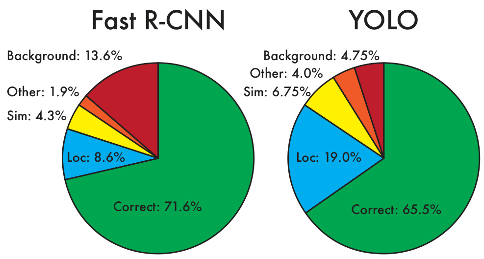
Because the two fail differently, they combine well. For every box Fast R-CNN predicts, the ensemble checks whether YOLO predicts a similar box, and if so boosts that prediction using YOLO’s probability and the overlap between the two boxes. The best Fast R-CNN model rises from 71.8% to 75.0% mAP, a gain of 3.2 points. Ensembling several versions of Fast R-CNN with each other gains only 0.3 to 0.6 points, which is the evidence that the gain comes from complementary error profiles rather than from averaging. The combination is not free in time — the two models run separately — but YOLO is fast enough that it adds no significant computation.
The structural limits are three, and each is a property of the design rather than of the training:
- Spatial constraints. Each grid cell predicts only two boxes and can have only one class. This caps the number of nearby objects the model can predict, and it is why groups of small objects, such as flocks of birds, fail.
- Coarse features. The architecture has multiple downsampling layers from the input image, so the features used for box prediction are relatively coarse. Boxes are learned entirely from data, so unusual aspect ratios and configurations generalise poorly.
- A loss that is only an approximation. The loss treats errors in small and large bounding boxes the same. A small error in a large box is generally benign, but a small error in a small box has a much greater effect on IoU.
What the design buys, beyond frame rate, is domain transfer. Trained on natural images and tested on artwork, YOLO reaches 53.3% AP with best \(F_1\) of 0.590 on the Picasso dataset, against 10.4% AP for R-CNN and 37.8% for DPM, and 45% AP on People-Art against 26% and 32%. R-CNN drops sharply because Selective Search is tuned for natural images and its classifier sees only small regions with good proposals. YOLO models the size and shape of objects and the relationships between them, and artwork differs from natural images at the pixel level while remaining similar in size and shape. Attached to a webcam, including the time to fetch and display images, the system holds real-time performance and functions as a tracking system.
Learning outcomes
- yolo-error-profile Diagnose a single-shot detector’s error profile and its structural limits.
- detector-design-tradeoffs Choose a detector for a deployment constraint by reasoning about speed, accuracy and object scale.
Concepts
- grid-based-prediction two boxes and one class per cell bound how many nearby objects can be reported at all
- fast-yolo 52.7% mAP at 155 frames per second on VOC 2007, twice the accuracy of the fastest prior real-time detector
- unified-object-detection a single evaluation makes latency independent of the number of objects, so no batching is needed for streaming video
- global-context-reasoning seeing the whole image while predicting each box cuts background false positives to 4.75%, against 13.6% for Fast R-CNN
- cross-domain-generalizability modelling object size and shape rather than local pixel statistics is what survives the move to artwork
SSD: default boxes across scales
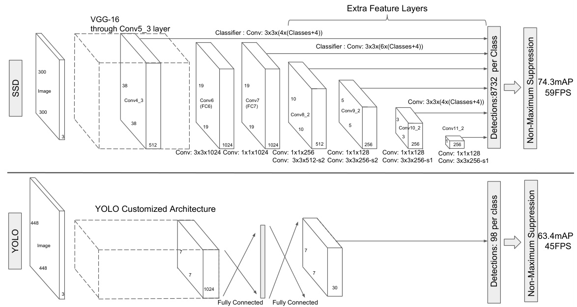
Liu et al. (2016) keep the single pass but change the prediction surface. The base network is an early truncated high-quality image classification network, VGG-16 in their experiments, with the classification layers removed. Auxiliary convolutional feature layers are then appended, decreasing in size progressively, and predictions are taken from several of them at once.
Convolutional predictors replace YOLO’s fully connected head. Each added feature layer, or an existing layer from the base network, produces a fixed set of detection predictions. For a feature layer of size \(m \times n\) with \(p\) channels, the basic element for predicting the parameters of a potential detection is a \(3 \times 3 \times p\) small kernel that produces either a score for a category, or a shape offset relative to the default box coordinates. At each of the \(m \times n\) locations where the kernel is applied, it produces an output value.
Default boxes are what the offsets are relative to. A set of default bounding boxes is associated with each feature map cell, tiled in a convolutional manner so the position of each box relative to its cell is fixed. For each of \(k\) boxes at a location, \(c\) class scores and 4 offsets relative to the original default box shape are computed. This gives \((c + 4)k\) filters applied around each location, and \((c + 4)kmn\) outputs for an \(m \times n\) feature map. The default boxes are similar to the anchor boxes of Faster R-CNN, applied to several feature maps of different resolutions.
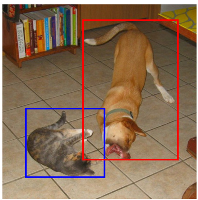
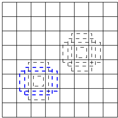
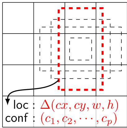
The scales are set by formula rather than by hand. For \(m\) feature maps used for prediction, the scale of the default boxes on the \(k\)th map is
\[s_k = s_{\min} + \frac{s_{\max} - s_{\min}}{m - 1}(k - 1), \qquad k \in [1, m],\]
with \(s_{\min} = 0.2\) and \(s_{\max} = 0.9\), so the lowest layer has scale 0.2, the highest 0.9, and everything between is regularly spaced. Aspect ratios \(a_r \in \{1, 2, 3, \tfrac{1}{2}, \tfrac{1}{3}\}\) give width \(w_k^a = s_k \sqrt{a_r}\) and height \(h_k^a = s_k / \sqrt{a_r}\). For the ratio 1 a further box of scale \(s'_k = \sqrt{s_k s_{k+1}}\) is added, yielding 6 default boxes per feature map location. The centre of each default box is \(\left(\frac{i + 0.5}{|f_k|}, \frac{j + 0.5}{|f_k|}\right)\) where \(|f_k|\) is the size of the \(k\)th square feature map.
Matching assigns ground truth to specific outputs, which is the key difference from training a proposal-based detector. Each ground-truth box is first matched to the default box with the best Jaccard overlap. Unlike MultiBox, matching then continues: default boxes are matched to any ground truth with overlap higher than 0.5. That simplifies the learning problem — the network may predict high scores for several overlapping default boxes rather than being required to pick the one with maximum overlap.
The objective is a weighted sum of the localisation and confidence losses,
\[L(x, c, l, g) = \frac{1}{N}\left(L_{conf}(x, c) + \alpha L_{loc}(x, l, g)\right),\]
where \(N\) is the number of matched default boxes and the loss is set to 0 if \(N = 0\). The localisation term is a smooth \(L_1\) loss between the predicted box \(l\) and the ground-truth box \(g\), regressing offsets for the centre \((cx, cy)\) of the default box \(d\) and for its width and height, with \(\hat{g}^{w}_j = \log(g^w_j / d^w_i)\) and likewise for the height. The confidence term is the softmax loss over class confidences, and \(\alpha\) is set to 1 by cross validation.
Learning outcomes
- ssd-multiscale-default-boxes Design a detector that predicts from default boxes tiled over feature maps of several resolutions.
Concepts
- single-shot-multibox-detector a feed-forward network producing a fixed-size collection of boxes and class scores, with no proposal stage and no feature resampling
- multi-scale-feature-maps auxiliary layers decreasing in size let a large object be matched on a coarse map and a small one on a fine map
- convolutional-predictors a \(3 \times 3 \times p\) kernel per prediction gives \((c+4)kmn\) outputs from an \(m \times n\) map, in place of a fully connected head
- default-boxes scales follow \(s_k = s_{\min} + \frac{s_{\max}-s_{\min}}{m-1}(k-1)\) and aspect ratios \(\{1, 2, 3, \tfrac12, \tfrac13\}\), and every offset is predicted relative to one of them
Making single-shot training work
After the matching step, most of the default boxes are negatives, especially when the number of possible default boxes is large. Hard negative mining answers that imbalance: instead of using all the negative examples, the negatives are sorted by their highest confidence loss for each default box and the top ones are picked, so that the ratio between negatives and positives is at most 3:1. Liu et al. (2016) report that this leads to faster optimisation and more stable training.
Augmentation is the second mechanism, and its effect is larger than the word “trick” suggests. Each training image is randomly sampled by one of the following options:
- Use the entire original input image.
- Sample a patch so that the minimum Jaccard overlap with the objects is 0.1, 0.3, 0.5, 0.7 or 0.9.
- Randomly sample a patch.
The size of each sampled patch is \([0.1, 1]\) of the original image size, and its aspect ratio is between \(\tfrac12\) and 2. The overlapped part of a ground-truth box is kept if the centre of it is in the sampled patch. Each patch is then resized to fixed size, horizontally flipped with probability 0.5, and photometrically distorted.
Those random crops act as a zoom in operation and generate larger training examples. Zoom-out augmentation supplies the opposite: the image is randomly placed on a canvas of \(16\times\) the original image size, filled with mean values, before the random crop step. Because this introduces more training images, the training iterations have to be doubled. The gain is a consistent 2–3% mAP across datasets, and it lands almost entirely on small objects — SSD300 rises from 74.3% to 77.2% on VOC 2007, and SSD512 from 26.8% to 28.8% mAP on COCO.
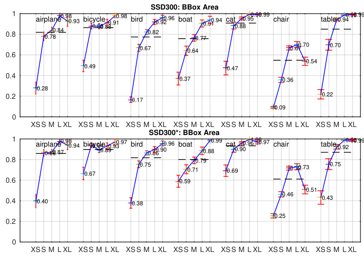
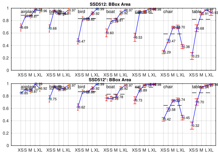
The ablations, all at \(300 \times 300\) input, attribute the accuracy:
- Augmentation raises VOC 2007 test mAP from 65.5% to 74.3%, a gain of 8.8 points — the largest single entry in the table.
- Removing the boxes with \(\tfrac13\) and 3 aspect ratios costs 0.6 points; removing \(\tfrac12\) and 2 as well costs another 2.1. A variety of default box shapes makes the task of predicting boxes easier for the network.
- The atrous version of the subsampled VGG-16 gives about the same result as the full VGG-16 with
pool5kept at \(2 \times 2 - s2\), while being about 20% faster.
The layer-count ablation is the one that matters most for design. Prediction layers are removed progressively, and each time the default box tiling is adjusted to keep the total near 8732 boxes. mAP drops monotonically from 74.3% with all six sources — conv4_3, conv7, conv8_2, conv9_2, conv10_2, conv11_2 — to 62.4% when only conv7 is used. Using primarily finer resolution maps starts increasing performance again once enough large boxes remain. It is the number of resolutions, not the number of boxes, that carries the accuracy.
Neither mechanism is incidental. The extreme background-to-object ratio and the weakness on small objects are consequences of predicting densely without resampling features, so any proposal-free detector inherits both problems and must answer them somehow.
Learning outcomes
- training-single-shot-detectors Stabilise single-shot training with hard negative mining and aggressive augmentation.
Concepts
- default-boxes matching gives each ground-truth box its best default box and every default box above 0.5 overlap, so several predictors are trained on one object
- hard-negative-mining negatives ranked by confidence loss and capped at 3:1 against the positives keeps the background from dominating the gradient
- multi-scale-feature-maps removing prediction layers while holding the box count fixed costs 11.9 mAP, so resolution diversity is what the accuracy rests on
- zoom-out-data-augmentation a \(16\times\) mean-filled canvas manufactures small training objects and is worth 2–3 mAP
SSD results and runtime
On VOC 2007 test, with 07+12 training data, SSD300 reaches 74.3% mAP against Faster R-CNN’s 73.2%, and SSD512 reaches 76.8%. Trained on COCO trainval35k and fine-tuned on 07+12, SSD512 reaches 81.6% mAP. On VOC 2012 test the ordering holds: SSD300 at 72.4% and SSD512 at 74.9% on 07++12, against Faster R-CNN’s 70.4% and YOLO’s 57.9%; with COCO pretraining SSD512 reaches 80.0%. Input resolution is the main knob — the two SSD models have exactly the same settings apart from their input size.
The error profile is specific. Using the detection analysis tool of Hoiem et al., SSD detects various object categories with high quality, and recall is around 85–90% under the weak (0.1 overlap) criterion. Compared with R-CNN, SSD has less localisation error, because it directly learns to regress the object shape and classify object categories instead of using two decoupled steps. It has more confusions with similar object categories, partly because locations are shared for multiple categories. And it is very sensitive to bounding box size: performance on small objects is much worse than on big ones, because those small objects may not even have any information at the very top layers. Raising the input from \(300 \times 300\) to \(512 \times 512\) helps, but does not close the gap.
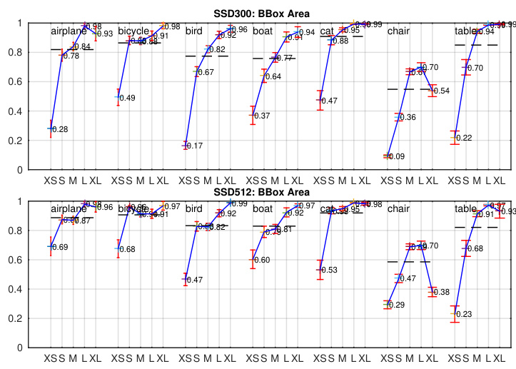
On COCO test-dev2015 the default boxes are made smaller, with \(s_{\min}\) reduced to 0.15 and the scale on conv4_3 set to 0.07 — about 21 pixels for a \(300 \times 300\) image. SSD512 reaches 26.8% AP at IoU 0.5:0.95, 46.5% at 0.5 and 27.8% at 0.75, against Faster R-CNN’s 24.2% and 45.3%. The margin is larger at the stricter threshold: SSD512 is 5.3% better at mAP@0.75 but only 1.2% better at mAP@0.5. It also has much better AP (4.8%) and AR (4.6%) for large objects, but relatively little improvement in AP (1.3%) and AR (2.0%) for small ones.
Runtime is where the design pays. With a confidence threshold of 0.01 most boxes are filtered out, then non-maximum suppression with Jaccard overlap 0.45 per class, keeping the top 200 detections per image, costs about 1.7 ms per image — close to the total 2.4 ms spent on all newly added layers. On a Titan X with cuDNN v4, SSD300 runs at 46 frames per second at batch size 1 and 59 at batch size 8, evaluating 8732 boxes per image; SSD512 runs at 19 and 22 frames per second on 24564 boxes. About 80% of the forward time is spent on the base network, so a faster base network would improve the speed further.
Faster R-CNN drew the opposite conclusion from its own dense-detection experiment. The assumption that changed is that dense prediction must come from a single resolution: SSD’s default boxes are Faster R-CNN’s anchors applied at several resolutions and without a proposal stage, and per-box class scores are produced directly rather than by pooling features and evaluating a separate classifier.
SSD300 is the first real-time method to achieve above 70% mAP. Fast YOLO runs at 155 frames per second but is almost 22% lower in mAP.
Key ideas
- Input resolution, not architecture, is the main accuracy-versus-speed control within one SSD design.
- The weakness is small objects, and the cause is that a coarse top-layer feature map carries little signal about them.
- The backbone dominates the forward pass; the box overhead and non-maximum suppression together are a few milliseconds.
Learning outcomes
- training-single-shot-detectors Stabilise single-shot training with hard negative mining and aggressive augmentation.
- detector-design-tradeoffs Choose a detector for a deployment constraint by reasoning about speed, accuracy and object scale.
Concepts
- single-shot-multibox-detector 74.3% mAP at 59 frames per second on VOC 2007 is the first case of a one-stage detector matching a two-stage one under equal training data
- default-boxes their scales are dataset-dependent, and COCO needs \(s_{\min}\) lowered to 0.15 because its objects are smaller than PASCAL’s
YOLOv2: better
Redmon and Farhadi (2017) treat the second version as a sequence of separately measured changes. Error analysis of YOLO compared to Fast R-CNN shows a significant number of localisation errors and relatively low recall against region-proposal methods, so the work is aimed at recall and localisation while maintaining classification accuracy. Rather than scaling up the network, the network is simplified and the representation made easier to learn. The path from 63.4% to 78.6% mAP on VOC 2007 runs as follows.
- Batch normalisation on all of the convolutional layers gives more than 2% improvement in mAP and also regularises the model, so dropout can be removed without overfitting.
- High-resolution classifier. The original YOLO trains the classifier at \(224 \times 224\) and raises the resolution to 448 for detection, so the network has to simultaneously switch to learning detection and adjust to the new input resolution. YOLOv2 first fine-tunes the classification network at the full \(448 \times 448\) resolution for 10 epochs on ImageNet, then fine-tunes the result on detection. This gives an increase of almost 4% mAP.
- Convolutional with anchor boxes. The fully connected layers are removed and anchor boxes predict bounding boxes instead. One pooling layer is eliminated to raise resolution, and the network is shrunk to operate on \(416 \times 416\) inputs rather than \(448 \times 448\), so that the \(13 \times 13\) output feature map has an odd number of locations and therefore a single centre cell — objects, especially large objects, tend to occupy the centre of the image. Class prediction is decoupled from spatial location: class and objectness are predicted for every anchor box, with objectness still predicting the IoU of the ground truth and the proposed box. The intermediate model gets 69.5% mAP with 81% recall without anchors, and 69.2% mAP with 88% recall with them. Accuracy decreases slightly while recall gains 7 points, which means the model has more room to improve.
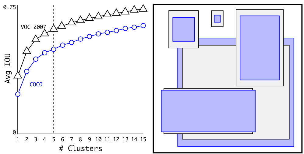
Dimension clusters replace hand-picked box shapes. \(k\)-means is run on the training set bounding boxes to find good priors automatically. Standard \(k\)-means with Euclidean distance would let larger boxes generate more error than smaller ones, so the distance metric is
\[d(\text{box}, \text{centroid}) = 1 - \mathrm{IOU}(\text{box}, \text{centroid}),\]
which depends on overlap rather than on box size. At \(k = 5\) the centroids give an average IoU of 61.0 against the closest prior, where 9 hand-picked anchor boxes give 60.9; nine centroids give 67.2. The clusters are significantly different from hand-picked anchors: there are fewer short, wide boxes and more tall, thin ones.
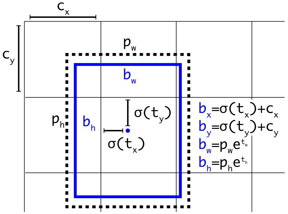
Direct location prediction fixes the remaining instability, which comes from predicting the \((x, y)\) locations. A region proposal network computes \(x = (t_x * w_a) - x_a\) and \(y = (t_y * h_a) - y_a\), which is unconstrained, so any anchor box can end up at any point in the image regardless of which location predicted the box. With random initialisation the model takes a long time to stabilise to sensible offsets. Instead, location coordinates are predicted relative to the grid cell and bounded by a logistic activation. With the cell offset by \((c_x, c_y)\) from the top left corner and a prior of width and height \(p_w, p_h\), the five coordinates \(t_x, t_y, t_w, t_h, t_o\) give
\[b_x = \sigma(t_x) + c_x, \quad b_y = \sigma(t_y) + c_y, \quad b_w = p_w e^{t_w}, \quad b_h = p_h e^{t_h},\] \[\Pr(\text{object}) * IOU(b, \text{object}) = \sigma(t_o).\]
Constraining the parameterisation makes it easier to learn and the network more stable. Dimension clusters together with directly predicting the box centre improve YOLO by almost 5% mAP over the version with anchor boxes.
Two changes remain. Fine-grained features: the \(13 \times 13\) map is sufficient for large objects but may benefit from finer features for localising smaller ones, so a passthrough layer brings features from an earlier layer at \(26 \times 26\). It concatenates the higher-resolution features with the low-resolution features by stacking adjacent features into different channels instead of spatial locations, similar to the identity mappings in ResNet, turning the \(26 \times 26 \times 512\) map into a \(13 \times 13 \times 2048\) map. This gives a modest 1% increase. Multi-scale training: since the model uses only convolutional and pooling layers it can be resized on the fly, so every 10 batches the network randomly chooses a new input dimension from the multiples of 32 between \(320 \times 320\) and \(608 \times 608\). The same weights then serve the whole curve — at \(288 \times 288\) YOLOv2 runs at more than 90 frames per second with mAP almost as good as Fast R-CNN, and at \(544 \times 544\) it reaches 78.6% mAP on VOC 2007 while still above real-time speed.
Learning outcomes
- yolov2-design-improvements Explain each YOLOv2 change and the mAP it contributes.
Concepts
- yolov2 a fully convolutional grid detector with clustered priors, reaching 78.6% mAP at 40 frames per second and 76.8% at 67
- dimension-clusters \(k\)-means under \(d = 1 - \mathrm{IOU}\) gives 5 priors that match the data better than 9 hand-picked anchors
- direct-location-prediction a sigmoid keeps a box centre inside the cell that predicted it, which removes the early instability of unbounded offsets
- multi-scale-training resampling the input size every 10 batches makes one set of weights usable across the whole speed-accuracy curve
YOLOv2: faster
Most detection frameworks of the period rely on VGG-16 as the base feature extractor. It is powerful and accurate, but needlessly complex: its convolutional layers require 30.69 billion floating point operations for a single pass over a single image at \(224 \times 224\) resolution. The original YOLO used a custom network based on the GoogLeNet architecture, which is faster at 8.52 billion operations per forward pass, with slightly worse accuracy — 88.0% single-crop top-5 on ImageNet against VGG-16’s 90.0%.
Darknet-19 is designed for the same job with fewer operations. Its construction follows established practice:
- Mostly \(3 \times 3\) filters, doubling the number of channels after every pooling step, as in the VGG models.
- \(1 \times 1\) convolutions to compress the representation between \(3 \times 3\) convolutions, following the Network in Network work, and global average pooling to make predictions.
- Batch normalisation throughout, to stabilise training, speed up convergence and regularise the model.
The final model has 19 convolutional layers and 5 maxpooling layers. It requires only 5.58 billion operations to process an image, yet achieves 72.9% top-1 and 91.2% top-5 accuracy on ImageNet.
Classification training runs on the standard ImageNet 1000-class dataset for 160 epochs using stochastic gradient descent with a starting learning rate of 0.1, polynomial rate decay with a power of 4, weight decay 0.0005 and momentum 0.9, in the Darknet framework, with random crops, rotations, and hue, saturation and exposure shifts. The network is then fine-tuned at 448 for 10 epochs starting at a learning rate of \(10^{-3}\), reaching 76.5% top-1 and 93.3% top-5 at that resolution.
Detection training modifies the network by removing the last convolutional layer and instead adding on three \(3 \times 3\) convolutional layers with 1024 filters each followed by a final \(1 \times 1\) convolutional layer with the number of outputs needed for detection. For VOC, five boxes with five coordinates each and 20 classes per box give 125 filters. The passthrough layer is added from the final \(3 \times 3 \times 512\) layer to the second to last convolutional layer, so the model can use fine-grained features. Training runs for 160 epochs starting at \(10^{-3}\), dividing by 10 at 60 and 90 epochs, with weight decay 0.0005 and momentum 0.9, and the same schedule is used on COCO and VOC.
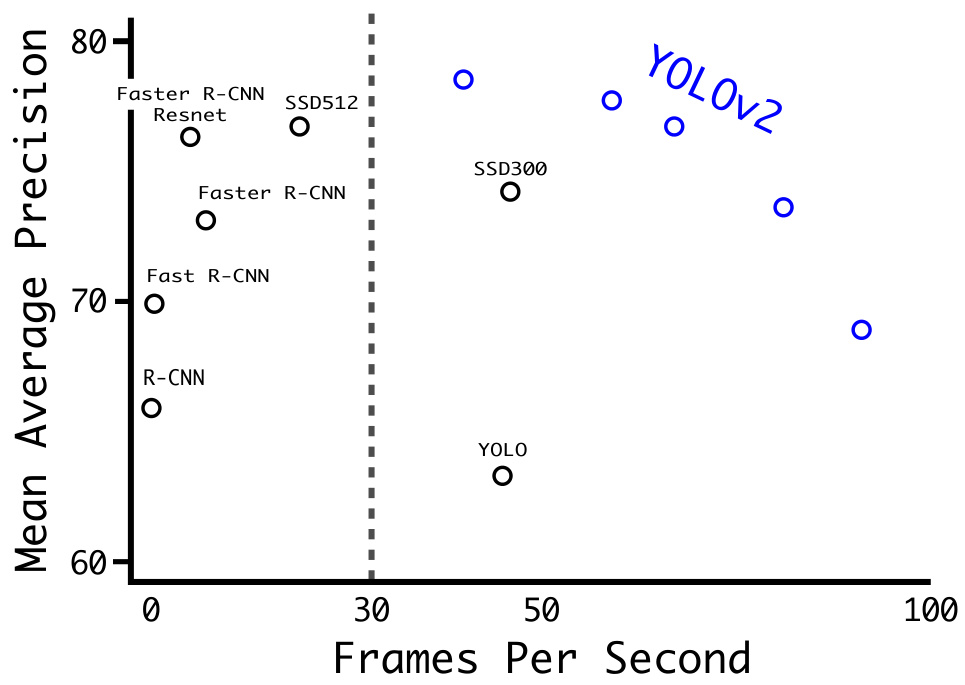
The speed comes from where the operations are. Reducing the backbone from 30.69 to 5.58 billion operations cut computation by 33% relative to the anchor-box intermediate model without changing the detection head’s design. The runtime breakdown of SSD says the same thing from the other side: about 80% of that forward pass is the base network too.
Learning outcomes
- yolov2-design-improvements Explain each YOLOv2 change and the mAP it contributes.
- detector-design-tradeoffs Choose a detector for a deployment constraint by reasoning about speed, accuracy and object scale.
Concepts
- darknet-19 19 convolutional and 5 maxpooling layers, 5.58 billion operations per image, 72.9% top-1 on ImageNet — against VGG-16’s 30.69 billion
- yolov2 detection training removes the last convolutional layer, adds three \(3 \times 3 \times 1024\) layers and a \(1 \times 1\) output layer sized for the priors and classes
YOLO9000: stronger
Detection datasets have only common objects and general labels, like “dog” or “boat”. Classification datasets have a much wider and deeper range: ImageNet has more than a hundred breeds of dog, including “Norfolk terrier”, “Yorkshire terrier” and “Bedlington terrier”. Training on both requires a coherent way to merge these labels, and a softmax layer across all possible categories cannot do it, because a softmax assumes the classes are mutually exclusive and “Norfolk terrier” and “dog” are not. A multi-label model that drops the exclusivity assumption would also discard the structure that is known — all of the COCO classes are mutually exclusive.
WordTree supplies the structure. ImageNet labels are pulled from WordNet, a language database that structures concepts and how they relate: “Norfolk terrier” and “Yorkshire terrier” are both hyponyms of “terrier”, which is a type of “hunting dog”, which is a type of “dog”, which is a “canine”. WordNet is a directed graph rather than a tree, because language is complex — a “dog” is both a type of “canine” and a type of “domestic animal” — so the problem is simplified by building a hierarchical tree from the concepts in ImageNet. The visual nouns are examined, their paths through the WordNet graph to the root node “physical object” are traced, and the paths that grow the tree by as little as possible are added iteratively: given two paths to the root, one adding three edges and one adding one, the shorter is chosen.
Classification with WordTree predicts a conditional probability at every node, for the probability of each hyponym of that synset given that synset. At the “terrier” node the predictions are \(\Pr(\text{Norfolk terrier} \mid \text{terrier})\), \(\Pr(\text{Yorkshire terrier} \mid \text{terrier})\), \(\Pr(\text{Bedlington terrier} \mid \text{terrier})\), and so on. The absolute probability of a node follows the path to the root and multiplies:
\[ \begin{aligned} \Pr(\text{Norfolk terrier}) = &\ \Pr(\text{Norfolk terrier} \mid \text{terrier}) \\ &* \Pr(\text{terrier} \mid \text{hunting dog}) * \ldots \\ &* \Pr(\text{mammal} \mid \text{animal}) * \Pr(\text{animal} \mid \text{physical object}), \end{aligned} \]
with \(\Pr(\text{physical object}) = 1\) assumed for classification. A hierarchical softmax is computed over all sysnsets that are hyponyms of the same concept, rather than one softmax over everything.
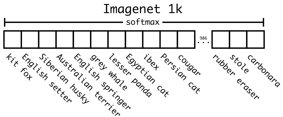
Building WordTree1k over ImageNet’s 1000 classes expands the label space from 1000 to 1369 nodes, and ground-truth labels are propagated up the tree during training, so an image labelled “Norfolk terrier” is also labelled “dog” and “mammal”. Hierarchical Darknet-19 achieves 71.9% top-1 and 90.4% top-5 accuracy — a marginal drop despite the 369 added concepts. It also degrades gracefully: shown a picture of a dog of uncertain breed, the network still predicts “dog” with high confidence and spreads lower confidences over the hyponyms.
Joint classification and detection training builds the dataset by mapping the categories of both sources onto tree synsets. COCO detection is combined with the top 9000 classes from the full ImageNet release, plus the ImageNet detection challenge classes not already included, for a WordTree of 9418 classes. ImageNet is much larger, so COCO is oversampled to bring the ratio to 4:1. The base YOLOv2 architecture is used with 3 priors instead of 5, to limit output size. The routing is the point:
- On a detection image, loss is backpropagated as normal.
- On a classification image, loss is backpropagated only at or above the corresponding level of the label. If the label is “dog”, no error is assigned to predictions further down the tree — “German Shepherd” against “Golden Retriever” — because that information is not available. The bounding box that predicts the highest probability for that class is found, and the loss is computed on just its predicted tree, with the objectness loss backpropagated under the assumption that the predicted box overlaps what would be the ground-truth label by at least 0.3 IoU.
YOLO9000 is evaluated on the ImageNet detection task, which shares only 44 object categories with COCO, so most of the test classes have been seen only as classification data. It gets 19.7 mAP overall, and 16.0 mAP on the disjoint 156 object classes it has never seen any labelled detection data for, while simultaneously detecting 9000 other categories in real time. Per-class results split sharply. Its best classes are animals: armadillo at 61.7, tiger at 61.0, koala bear at 54.3. Its worst are 0.0 for diaper, horizontal bar, rubber eraser, sunglasses and swimming trunks. New animals are easier to learn because the objectness predictions generalise well from the animals in COCO; COCO has no bounding box label for any type of clothing, only for person, so categories like “sunglasses” or “swimming trunks” have nothing to transfer from.
Learning outcomes
- joint-training-large-vocabulary Combine detection and classification data over a label hierarchy to detect thousands of classes.
Concepts
- wordtree a tree over WordNet synsets on which class probability is the product of conditionals along the path to “physical object”
- joint-training-algorithm localisation is learned from the detection dataset and naming from the classification dataset, with the classification loss applied only at or above the labelled node
- yolo9000 9418 classes in real time, 19.7 mAP on ImageNet detection and 16.0 mAP on the 156 classes with no box labels at all
Feature pyramid networks
Recognising objects at vastly different scales is a fundamental challenge, and Lin et al. (2017) set out four ways of meeting it. The four are worth holding separately, because the differences between them are the whole argument.
- Featurised image pyramid. Features are computed on each of the image scales independently. The pyramid is scale-invariant in the sense that an object’s scale change is offset by shifting its level, and each level is semantically strong including at high resolution. Inference time increases considerably — by four times in one reported case — and training end-to-end on an image pyramid is infeasible in terms of memory, so image pyramids are used only at test time, which creates an inconsistency between train-time and test-time inference.
- Single feature map. What Fast and Faster R-CNN opt for by default. Fast, and a good trade-off between accuracy and speed, but multi-scale detection still performs better, especially for small objects.
- Pyramidal feature hierarchy. A deep ConvNet already computes a feature hierarchy layer by layer, with a multi-scale, pyramidal shape. Reusing it would come free of cost. But its high-resolution maps have low-level features that harm their representational capacity for object recognition. SSD is one of the first attempts at using this hierarchy as if it were a featurised image pyramid, and to avoid using low-level features it foregoes reusing already computed layers and instead starts from high up in the network, at
conv4_3of VGG, adding several new layers. It thus misses the opportunity to reuse the higher-resolution maps of the feature hierarchy. - Feature pyramid network. A pyramid that has strong semantics at all levels and is built quickly from a single input image scale.
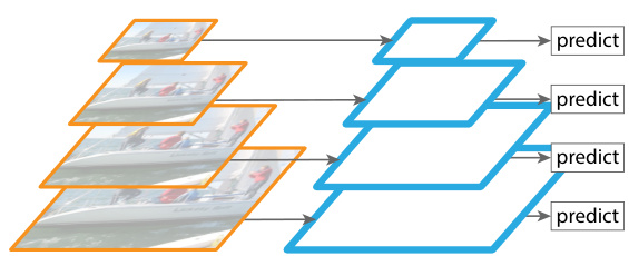
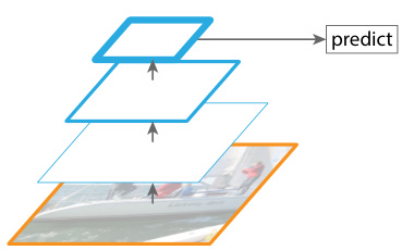
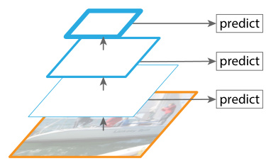
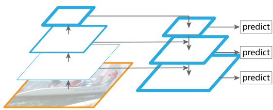
A related family of architectures — U-Net, SharpMask, recombinator networks, stacked hourglass networks — adopts top-down and skip connections, but its goal is to produce a single high-level feature map of a fine resolution on which predictions are made. The feature pyramid network uses the same architecture as a feature pyramid, with predictions made independently at each level.
The construction has three parts. The bottom-up pathway is the feed-forward computation of the backbone. One pyramid level is defined for each stage, since the deepest layer of each stage should have the strongest features. For ResNets, the output of the last residual block of each stage gives \(\{C_2, C_3, C_4, C_5\}\) for the conv2 through conv5 outputs, with strides \(\{4, 8, 16, 32\}\) with respect to the input image. conv1 is not included, because of its large memory footprint.
The top-down pathway hallucinates higher resolution features by upsampling spatially coarser but semantically stronger feature maps from higher pyramid levels, by a factor of 2 using nearest neighbour upsampling for simplicity. The lateral connections enhance those features with features from the bottom-up pathway. Each lateral connection merges feature maps of the same spatial size from the two pathways: the bottom-up map is of lower-level semantics, but its activations are more accurately localised as it was subsampled fewer times. The merge is element-wise addition, after the bottom-up map passes through a \(1 \times 1\) convolutional layer to reduce channel dimensions.
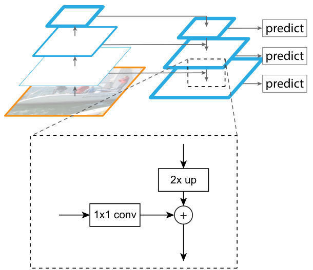
Iteration starts by attaching a \(1 \times 1\) convolutional layer on \(C_5\) to produce the coarsest resolution map, and continues until the finest resolution map is generated. A \(3 \times 3\) convolution is appended on each merged map to generate the final feature map, which reduces the aliasing effect of upsampling. The result is \(\{P_2, P_3, P_4, P_5\}\), of the same spatial sizes as \(\{C_2, C_3, C_4, C_5\}\).
Because all levels of the pyramid use shared classifiers and regressors as in a traditional featurised image pyramid, the feature dimension is fixed at \(d = 256\) in all the feature maps, so all extra convolutional layers have 256-channel outputs. There are no non-linearities in these extra layers, which was found empirically to have minor impacts.
Learning outcomes
- feature-pyramid-construction Build an in-network feature pyramid with a top-down pathway and lateral connections.
Concepts
- feature-pyramid-network one backbone pass plus thin convolutional layers yields a pyramid with strong semantics at every level, and predictions are made independently on each
- bottom-up-pathway one level per backbone stage, taken from the last residual block, giving \(\{C_2, \ldots, C_5\}\) at strides 4 to 32
- top-down-pathway-lateral-connections \(2\times\) nearest-neighbour upsampling merged by addition with a \(1 \times 1\)-reduced same-resolution map, then a \(3 \times 3\) convolution against aliasing
Attaching heads to the pyramid
The pyramid is a modification to the backbone, not a new detector, so both heads of the previous unit’s two-stage system attach to it with minimal modification.
FPN for RPN. In the original RPN a small subnetwork is evaluated on dense \(3 \times 3\) sliding windows on top of a single-scale convolutional feature map, performing object/non-object binary classification and bounding box regression, realised as a \(3 \times 3\) convolutional layer followed by two sibling \(1 \times 1\) convolutions. That same head is attached to each level of the feature pyramid. Because the head slides densely over all locations in all pyramid levels, it is not necessary to have multi-scale anchors on a specific level. Anchors of a single scale are assigned to each level instead: areas of \(\{32^2, 64^2, 128^2, 256^2, 512^2\}\) pixels on \(\{P_2, P_3, P_4, P_5, P_6\}\) respectively, with aspect ratios \(\{1{:}2, 1{:}1, 2{:}1\}\) at each level, so 15 anchors over the pyramid. (\(P_6\) is a stride-two subsampling of \(P_5\), present only to cover the \(512^2\) anchor scale, and it is not used by the Fast R-CNN detector.)
Training labels are assigned by IoU with ground truth as before: positive if an anchor has the highest IoU for a given ground-truth box or an IoU over 0.7 with any, negative if its IoU is below 0.3 for all. The scales of the ground-truth boxes are not used to assign them to pyramid levels; the boxes are associated with anchors, and the anchors have been assigned to levels.
The head’s parameters are shared across all levels. An unshared variant was evaluated and gave similar accuracy. That result is itself evidence about the pyramid: the good performance of sharing parameters indicates that all levels of the pyramid share similar semantic levels, which is the same advantage a featurised image pyramid has, where a common head classifier can be applied to features computed at any image scale.
FPN for Fast R-CNN. Fast R-CNN uses RoI pooling to extract features, and is most commonly performed on a single-scale map, so RoIs must be assigned to pyramid levels. Viewing the pyramid as if it were produced from an image pyramid, an RoI of width \(w\) and height \(h\) on the input image goes to level \(P_k\) by
\[k = \left\lfloor k_0 + \log_2\!\left(\sqrt{wh}/224\right) \right\rfloor.\]
Here 224 is the canonical ImageNet pre-training size, and \(k_0\) is the target level on which an RoI with \(w \times h = 224^2\) should be mapped into. Following the ResNet-based Faster R-CNN system, which uses \(C_4\) as the single-scale feature map, \(k_0\) is set to 4. Intuitively, if the RoI’s scale becomes smaller — say \(1/2\) of 224 — it should be mapped into a finer-resolution level, here \(k = 3\). Predictor heads attach to all RoIs of all levels and again share parameters. Where a ResNet’s conv5 layers are usually adopted as the head, that stage is already harnessed to build the pyramid, so RoI pooling extracts \(7 \times 7\) features and two hidden 1024-d fully connected layers with ReLU precede the classification and box regression layers — a lighter and faster head, randomly initialised since no pre-trained fully connected layers are available in ResNets.
The RPN ablations on COCO minival show that both halves of the pyramid design are load-bearing. Against a single-scale baseline on \(C_4\) with 5 scale anchors, adding FPN raises \(\mathrm{AR}^{1k}\) from 48.3 to 56.3, a gain of 8.0 points, and \(\mathrm{AR}^{1k}_s\) on small objects from 32.0 to 44.9, a gain of 12.9. A baseline on \(C_5\) shows no advantage over the one on \(C_4\), indicating that a single higher-level feature map is not enough, because there is a trade-off between coarser resolutions and stronger semantics. The two removals are decisive:
- Without the top-down pathway — \(1 \times 1\) lateral connections followed by \(3 \times 3\) convolutions attached to the bottom-up pyramid, simulating the pyramidal feature hierarchy — \(\mathrm{AR}^{1k}\) falls to 49.5, on par with the baseline. The conjecture is that there are large semantic gaps between different levels on a bottom-up pyramid, especially for very deep ResNets. An unshared-head variant of this configuration degraded similarly, so the problem cannot be remedied by level-specific heads.
- Without the lateral connections, \(\mathrm{AR}^{1k}\) falls to 46.1. The top-down pyramid then has strong semantic features and fine resolutions, but the locations of those features are not precise, because the maps have been downsampled and upsampled several times.
- Attaching the head to \(P_2\) alone — the highest-resolution, strongly semantic level, with all anchors assigned to it — gives 51.3. Better than the baseline, inferior to the full pyramid, and this variant uses far more anchors, 750k against 200k. Scanning over pyramid levels increases robustness to scale variance in a way that a larger number of anchors does not.
Learning outcomes
- fpn-in-a-detector Attach an RPN and a Fast R-CNN head to a feature pyramid, and read the ablations that justify it.
Concepts
- fpn-rpn-adaptation one anchor scale per level with three aspect ratios, 15 anchors over the pyramid, and a head whose parameters are shared across levels
- feature-pyramid-network the pyramid replaces the single-scale feature map in both heads without changing either loss or the training recipe
- scale-based-roi-assignment \(k = \lfloor k_0 + \log_2(\sqrt{wh}/224)\rfloor\) with \(k_0 = 4\) routes small RoIs to fine levels and large ones to coarse levels
- top-down-pathway-lateral-connections removing the top-down pathway costs 6.8 \(\mathrm{AR}^{1k}\) and removing the laterals costs 10.2, so semantics and precise localisation are supplied by different halves
- bottom-up-pathway used alone as a pyramid it performs at baseline level, because the semantic gap between its levels is large in a deep ResNet
FPN results and reach
Three experiments separate what the pyramid contributes from what better proposals contribute.
Fast R-CNN on fixed proposals. The proposals are frozen — those computed by RPN on FPN — so that only the region-based detector varies. With ResNet-50, FPN reaches 33.9 AP on COCO minival, against 31.9 AP for the standard conv5 head baseline on \(C_4\) and 28.8 AP for a baseline exploiting a 2-fc MLP head similar to the one used with the pyramid. Small-object AP rises 2.1 points over the conv5 baseline. That the 2-fc head is worse on its own is what makes the comparison meaningful: the lighter head gives no orthogonal advantage, so the 5.1-point gap over it is the pyramid’s. Removing the top-down connections drops AP to 24.9, a loss of 9.0 points, which says that a region classifier suffers severely when it must rely on low-level features at high resolutions. Using \(P_2\) alone gives 33.4 AP, only marginally worse than the full pyramid at 33.9, because RoI pooling is a warping-like operation and is therefore less sensitive to the region’s scale.
Faster R-CNN on consistent proposals. With RPN and the detector sharing the same backbone, FPN improves on a strong reproduction of the ResNet-50 baseline by 2.3 points AP and 3.8 points AP@0.5. That baseline is itself stronger than the originally published figure, for four identifiable reasons — an image scale of 800 pixels rather than 600, 512 RoIs per image rather than 64, 5 scale anchors rather than 4, and 1000 test-time proposals rather than 300 — and the honest comparison is the controlled one against it, not the 7.6-point margin over the published number. With feature sharing under 4-step training, inference takes 0.148 seconds per image on a single NVIDIA M40 GPU with ResNet-50 and 0.172 with ResNet-101, against 0.32 seconds for the single-scale ResNet-50 baseline. The extra lateral layers cost something; the lighter head more than pays for them.
Against the competition winners. With the number of mini-batches doubled at each learning rate, single-model ResNet-101 FPN reaches 36.2 AP and 59.1 AP@0.5 on COCO test-dev. The single-model entries it exceeds are AttractioNet at 35.7 AP, Faster R-CNN+++ at 34.9 and G-RMI at 34.7 — the 2015 and 2016 challenge winners. The two winning entries that used image pyramids at test time are exactly the ones the pyramid replaces. Iterative regression, hard negative mining, context modelling, stronger data augmentation and heavy ensembling are all absent, and are noted as complementary improvements that should boost accuracy further.
Segmentation proposals. The same pyramid generates instance segments, following the DeepMask and SharpMask framework, with \(d = 128\). A small \(5 \times 5\) MLP predicts \(14 \times 14\) masks and object scores in a fully convolutional fashion on each pyramid level, and a second MLP of input size \(7 \times 7\) handles half octaves, the two playing a role analogous to anchors in RPN. Mask scales \(\{32, 64, 128, 256, 512\}\) map to \(\{P_2, \ldots, P_6\}\), with 25% padding around the canonical object size. On the first 5k COCO val images, using both MLPs together reaches 45.7 AR; doubling the mask output resolution from \(14 \times 14\) to \(28 \times 28\) adds a point, and doubling the training iterations brings it to 48.1 AR. DeepMask reaches 37.1 and SharpMask 39.8, so the margin is over 8.3 points AR, and small-object AR nearly doubles from 17.4 to 32.6. The runtime is 0.15–0.25 seconds against 0.49–0.77, because the existing methods densely sample image pyramids and this one does not.
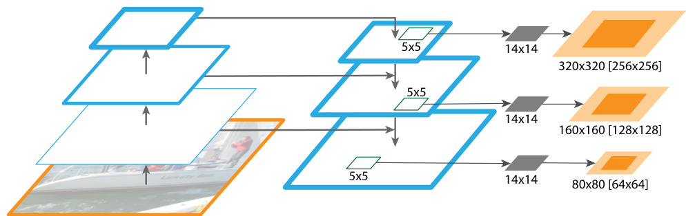
Both SSD and FPN are multi-scale, and the difference is which maps they predict from. SSD skips the backbone’s fine layers because they are semantically weak; FPN keeps them and repairs their semantics from above. The small-object numbers follow that distinction directly.
Learning outcomes
- fpn-in-a-detector Attach an RPN and a Fast R-CNN head to a feature pyramid, and read the ablations that justify it.
- detector-design-tradeoffs Choose a detector for a deployment constraint by reasoning about speed, accuracy and object scale.
Concepts
- scale-based-roi-assignment routing RoIs by size gives 33.9 AP against 31.9 for pooling everything from one map, holding the proposals fixed
- top-down-pathway-lateral-connections removing the top-down connections costs a region classifier 9.0 AP, far more than it costs a sliding-window proposer
- feature-pyramid-network 36.2 AP on COCO
test-devfrom a plain Faster R-CNN, at 0.148 seconds per image, without multi-scale testing or ensembling - fpn-segmentation-proposals the same pyramid drives a mask predictor to 48.1 AR at 6–7 frames per second, which is what makes it a general backbone rather than a detection trick
Choosing a detector
Three quantities span the design space these four papers cover, and each buys something at a stated price.
- Stages. Removing the second stage removes a per-region network evaluation. YOLO’s 45 frames per second and Fast YOLO’s 155 come from that, at 63.4% and 52.7% mAP on VOC 2007 against Faster R-CNN VGG-16’s 73.2% at 7 frames per second. SSD300’s 74.3% at 59 frames per second shows the accuracy cost is not intrinsic to having one stage.
- Input resolution. The main knob within one architecture, and the most expensive. SSD300 to SSD512 is 74.3% to 76.8% mAP and 59 to 22 frames per second. YOLOv2 at \(288 \times 288\) runs above 90 frames per second and at \(544 \times 544\) reaches 78.6% mAP, from one set of weights.
- Multi-scale features. The cheapest of the three. FPN costs one backbone pass and a handful of 256-channel convolutional layers, and its FPN-based Faster R-CNN is faster than the single-scale baseline it beats, 0.148 seconds against 0.32.
Object size decides between the last two. A detector predicting from a single coarse map has little signal about small objects at all: SSD’s sensitivity analysis is much worse on small objects than on large, its COCO gains over Faster R-CNN are 4.8% AP for large objects against 1.3% for small, and FPN’s largest margins are on exactly that class of object — 12.9 points of small-object recall for proposals, and nearly doubled small-object AR for masks.
Key ideas
Detection can be one regression from image pixels to boxes and class probabilities, evaluated once per image, and trained on a loss that is a loss on detection performance.
That is what makes latency independent of the number of objects, and what allows the whole image to be visible when each box is predicted.
A proposal-free detector has to solve two problems the proposal stage used to solve for it: assigning a predictor to each object, and surviving a background-to-object ratio in the hundreds.
YOLO answers with a responsible-predictor rule and \(\lambda_{\text{noobj}} = 0.5\); SSD answers with overlap-based matching and 3:1 hard negative mining. Learn the two problems, not either formula.
Seeing the whole image at once cuts background false positives to 4.75% against Fast R-CNN’s 13.6%, and costs localisation precision — 19.0% against 8.6%.
Because the two profiles are complementary, using YOLO to rescore Fast R-CNN gains 3.2 mAP where ensembling Fast R-CNN with itself gains 0.6.
Anchor priors are better obtained from the data than by hand, and better constrained than left free.
Five \(k\)-means centroids under \(d = 1 - \mathrm{IOU}\) match the training boxes as well as nine hand-picked anchors; a sigmoid on the centre offset removes the instability of letting any anchor land anywhere.
Detection vocabulary can be extended with data that has no boxes, by making the label space a tree and the classification loss apply only at or above the labelled node.
YOLO9000 reaches 16.0 mAP on 156 classes with no box labels at all, and 0.0 AP on clothing, because COCO has boxes for animals and none for clothes.
A feature map can be fine-resolution and semantically strong at the same time, if strong semantics are brought down to it.
Removing the top-down pathway costs 6.8 \(\mathrm{AR}^{1k}\) and removing the lateral connections 10.2, so neither half is decoration. Better features beat more machinery: 36.2 AP without multi-scale testing, iterative regression or ensembles.
The backbone dominates the forward pass in every one of these systems — about 80% of SSD’s, and 30.69 billion operations of VGG-16’s against Darknet-19’s 5.58.
Detection throughput is therefore a backbone design problem before it is a head design problem.
This closes the Computer Vision module. The three ideas carried forward are a shared backbone, a set of reference boxes, and a multi-task loss over classification and localisation.
References
Redmon, J., Divvala, S., Girshick, R., & Farhadi, A. (2016). You only look once: Unified, real-time object detection. In Proceedings of the IEEE conference on computer vision and pattern recognition (pp. 779-788).
Liu, W., Anguelov, D., Erhan, D., Szegedy, C., Reed, S., Fu, C. Y., & Berg, A. C. (2016, September). Ssd: Single shot multibox detector. In European conference on computer vision (pp. 21-37). Cham: Springer International Publishing.
Redmon, J., & Farhadi, A. (2017, July). YOLO9000: better, faster, stronger. In 2017 IEEE conference on computer vision and pattern recognition (CVPR) (pp. 6517-6525). IEEE.
Lin, T. Y., Dollár, P., Girshick, R., He, K., Hariharan, B., & Belongie, S. (2017, July). Feature pyramid networks for object detection. In 2017 IEEE conference on computer vision and pattern recognition (CVPR) (pp. 936-944). IEEE.