Lecture notes — Residual Convolutional Networks
ver. 1.1.0, residual_convolutional_networks
← Residual Convolutional Networks
ver. 1.1.0 · 2026-09-02 08:25:08
Where this fits
The previous unit established that depth is worth having and that it is fragile. VGG improved monotonically from 11 to 19 weight layers but had to initialise its deep configurations from a trained shallow one; GoogLeNet attached auxiliary classifiers to intermediate layers so that gradient would reach them. Both are devices for getting a deep network to train at all, not accounts of why it does not.
Two questions follow from that. The first is what actually obstructs depth, and whether it can be removed rather than worked around. The second is the reverse question: at a fixed accuracy, how little can a network cost in parameters, in multiply-adds, and in latency. Four papers answer these, and two tools carried over from the previous unit — the \(1\times1\) convolution for channel mixing and dimension reduction, and global average pooling in place of a fully connected head — appear in every one of them.
Learning outcomes
diagnose-the-degradation-problem— Diagnose the degradation problem and distinguish it from overfitting and from vanishing gradients.build-residual-blocks— Build residual blocks with identity shortcuts and justify the reformulation.assemble-deep-resnet-architectures— Assemble ResNet-18 through ResNet-152 using basic and bottleneck blocks.analyze-depth-empirically— Read the empirical evidence that residual networks gain accuracy from depth, and see where it stops.design-under-a-parameter-budget— Design a CNN under a hard parameter budget using squeeze-and-expand modules.explore-an-architecture-design-space— Explore a CNN design space through metaparameters rather than one-off architectures.build-densely-connected-blocks— Build a dense block where every layer receives the concatenated features of all preceding layers.explain-feature-reuse-and-implicit-supervision— Explain dense connectivity’s effects: feature reuse, implicit deep supervision, and regularization.use-depthwise-separable-convolutions— Factor a standard convolution into depthwise and pointwise stages and compute the saving.tune-width-and-resolution-multipliers— Trade accuracy for latency and size with the width multiplier \(\alpha\) and resolution multiplier \(\rho\).
Concepts introduced
- Degradation problem — adding layers to a suitably deep plain network raises its training error.
- Residual learning — stacked layers fit \(F(x) := H(x) - x\) instead of the target mapping \(H(x)\).
- Identity shortcut connection — a parameter-free skip that adds the block input to the block’s residual output.
- Bottleneck building block — a three-layer residual unit \(1\times1 \to 3\times3 \to 1\times1\) that reduces and then restores channel dimension.
- Dense connectivity — layer \(\ell\) takes the channel concatenation of every preceding layer in its block as input.
- Growth rate — the fixed number \(k\) of feature maps each dense layer contributes.
- Transition layers — the batch-normalisation, \(1\times1\) convolution and \(2\times2\) average pooling placed between dense blocks.
- DenseNet-BC — dense blocks with \(1\times1\) bottlenecks and transition outputs compressed by \(\theta\).
- Implicit deep supervision — every layer sits within a few transitions of the classifier, so it receives loss gradient directly.
- Feature reuse — later layers read early feature maps rather than re-deriving them.
- SqueezeNet — a Fire-module network reaching AlexNet accuracy at 4.8MB.
- Fire module — a \(1\times1\) squeeze layer feeding an expand layer of mixed \(1\times1\) and \(3\times3\) filters.
- Squeeze layer — the \(1\times1\) layer that reduces the channel count reaching \(3\times3\) filters.
- Expand layer — the parallel \(1\times1\) and \(3\times3\) filters whose outputs are concatenated.
- Squeeze ratio — the metaparameter \(SR = s_{1\times1}/(e_{1\times1}+e_{3\times3})\).
- Delayed downsampling — placing the strided layers late so most layers see large activation maps.
- Bypass connections in SqueezeNet — shortcut paths around Fire modules, simple or with a \(1\times1\) projection.
- Depthwise separable convolution — a depthwise spatial stage followed by a pointwise \(1\times1\) stage.
- Depthwise convolution — one \(D_K \times D_K\) filter per input channel, with no channel mixing.
- Pointwise convolution — a \(1\times1\) convolution that forms linear combinations across channels.
- Width multiplier — the factor \(\alpha\) that thins every layer’s channel count.
- Resolution multiplier — the factor \(\rho\) that shrinks the input resolution and every internal feature map.
- MobileNet architecture — 28 layers of depthwise separable blocks, batch normalisation and ReLU throughout.
The degradation problem
He, Kaiming, et al. “Deep residual learning for image recognition” (CVPR 2016) opens by separating three failures that are routinely confused.
The degradation problem is the observation that adding more layers to a suitably deep plain model leads to higher training error. On CIFAR-10 a 56-layer plain network has higher training error, and consequently higher test error, than a 20-layer one throughout training.
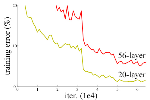
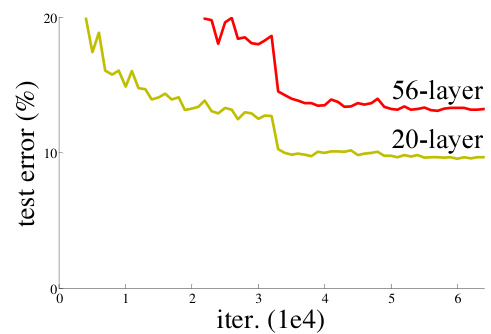
Three candidate explanations are ruled out in turn.
Not overfitting.
The gap appears in training error. A model that is overfitting fits its training set better, not worse.
Not vanishing or exploding gradients.
These were “largely addressed by normalized initialization and intermediate normalization layers”, which “enable networks with tens of layers to start converging for stochastic gradient descent (SGD) with backpropagation”. The plain networks here are trained with batch normalisation, “which ensures forward propagated signals to have non-zero variances”; the authors also verify that the backward propagated gradients “exhibit healthy norms with BN”. Neither the forward nor the backward signal vanishes.
Not a matter of training longer.
Experiments with three times the training iterations still show degradation, so the problem “cannot be feasibly addressed by simply using more iterations”.
What remains is optimisation. The argument is a construction. Take a shallower architecture and its deeper counterpart that adds layers onto it. There exists a solution by construction to the deeper model: the added layers compute the identity mapping, and the other layers are copied from the learned shallower model. That solution has training error no higher than the shallower model’s. Experiments show that solvers on hand are unable to find solutions comparably good or better than the constructed solution, or unable to do so in feasible time. The difficulty is therefore in the search, not in the hypothesis class. The authors’ conjecture is that deep plain nets “may have exponentially low convergence rates”.
Section 2 of the paper places this against earlier practice. Residual formulations were already known to ease optimisation elsewhere: VLAD and the Fisher Vector encode by residual vectors with respect to a dictionary, and the Multigrid method for partial differential equations reformulates a system as subproblems responsible for the residual solution between a coarser and a finer scale, converging much faster than standard solvers unaware of the residual nature of the solutions. Shortcut connections were also known: a linear layer connected from network input to output in MLP training, and the auxiliary classifiers of the previous unit. The concurrent highway networks use gating functions that are data-dependent and have parameters, and when a gated shortcut is “closed” (approaching zero) the layers represent non-residual functions.
The shortcuts introduced next differ on exactly that point: they carry no parameters and are never closed, so all information is always passed through.
Learning outcomes
- diagnose-the-degradation-problem Diagnose the degradation problem and distinguish it from overfitting and from vanishing gradients.
Concepts
- degradation-problem adding layers to a suitably deep plain network raises its training error, and a construction shows that a no-worse solution exists but is not found
Residual blocks and identity shortcuts
Let \(H(x)\) denote the underlying mapping to be fit by a few stacked layers, with \(x\) the input to the first of them. If stacked nonlinear layers can asymptotically approximate \(H(x)\), they can equally approximate the residual \(H(x) - x\), assuming input and output have the same dimensions. Residual learning takes the second option: the layers explicitly approximate
\[F(x) := H(x) - x,\]
and the original function becomes \(F(x) + x\).
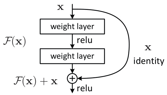
The motivation is the degradation problem. If the added layers can be constructed as identity mappings, a deeper model should have training error no greater than its shallower counterpart; degradation suggests the solvers have difficulty in approximating identity mappings by multiple nonlinear layers. Under the reformulation, if identity mappings are optimal the solvers may simply drive the weights of the multiple nonlinear layers toward zero. In real cases identity mappings are unlikely to be optimal, but the reformulation preconditions the problem: if the optimal function is closer to an identity mapping than to a zero mapping, it is easier for the solver to find the perturbations with reference to an identity mapping than to learn the function as a new one.
The building block is defined as
\[y = F(x, \{W_i\}) + x. \tag{1}\]
For the two-layer example, \(F = W_2\sigma(W_1 x)\) where \(\sigma\) denotes ReLU, and biases are omitted to simplify notation. The addition \(F + x\) is performed by a shortcut connection and element-wise addition, and the second nonlinearity is applied after the addition, giving \(\sigma(y)\). For convolutional layers the element-wise addition is performed on two feature maps, channel by channel.
Three properties follow, each of which matters for the experiments.
The shortcut in Eqn. (1) introduces neither extra parameter nor computation complexity.
This makes the comparison in the next section possible: plain and residual networks can be compared that simultaneously have the same number of parameters, depth, width, and computational cost, except for the negligible element-wise addition.
Dimension changes need a choice.
When the input and output channels differ, a linear projection \(W_s\) may be performed by the shortcut connections to match the dimensions: \(y = F(x, \{W_i\}) + W_s x\). Zero-padding the extra channels is the alternative and remains parameter-free. Identity mapping is sufficient for addressing the degradation problem and is economical, so \(W_s\) is used only when matching dimensions.
Granularity has a lower bound.
\(F\) in the paper’s experiments has two or three layers. If \(F\) has only a single layer, Eqn. (1) is similar to a linear layer, \(y = W_1 x + x\), for which no advantage has been observed.
The last point is the one most easily got wrong. The benefit does not come from the addition itself; a shortcut across one weight layer merely reparameterises a linear map. It comes from the residual branch being a stack of nonlinear layers whose target has been shifted to zero.
Learning outcomes
- build-residual-blocks Build residual blocks with identity shortcuts and justify the reformulation.
Concepts
- residual-learning stacked layers approximate \(F(x) := H(x) - x\), so driving the weights to zero yields an identity mapping and small perturbations of it are what the solver has to find
- identity-shortcut-connection the input is carried across the block and added element-wise, adding no parameters and no computation complexity, which makes plain and residual networks directly comparable
- degradation-problem the reformulation exists to remove it: an identity mapping is now trivial for the solver to represent
ResNet architectures and bottlenecks
The plain baselines are mainly inspired by the philosophy of VGG nets. The convolutional layers mostly have \(3\times3\) filters and follow two design rules: for the same output feature map size, the layers have the same number of filters; and if the feature map size is halved, the number of filters is doubled so as to preserve the time complexity per layer. Downsampling is performed directly by convolutional layers that have a stride of 2. The network ends with a global average pooling layer and a 1000-way fully connected layer with softmax. The 34-layer plain baseline has 3.6 billion FLOPs (multiply-adds), which is only 18% of VGG-19’s 19.6 billion.
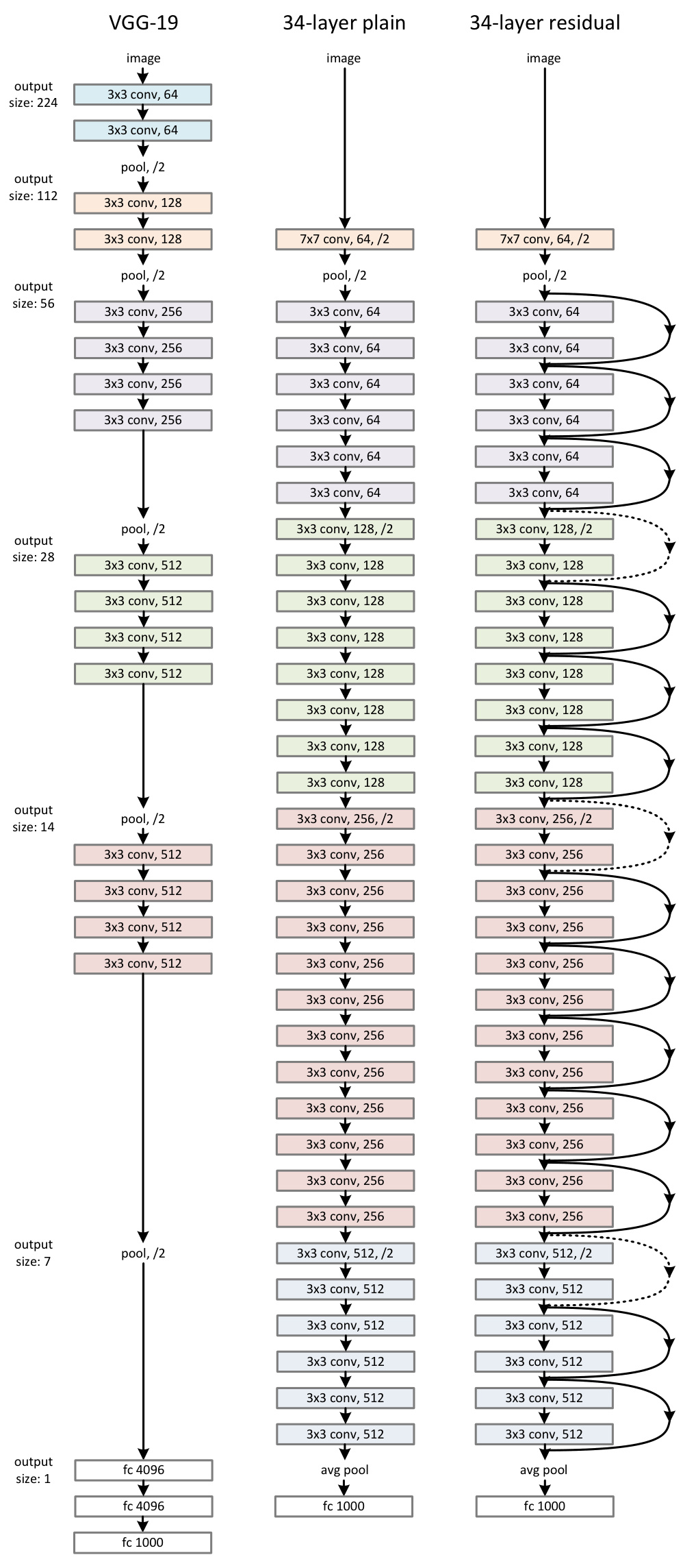
The residual version inserts shortcut connections into that same network. Identity shortcuts are used directly when input and output are of the same dimensions. When the dimensions increase, two options are considered: (A) the shortcut still performs identity mapping, with extra zero entries padded for increasing dimensions, which introduces no extra parameter; (B) the projection shortcut of Eqn. (2) is used to match dimensions, done by \(1\times1\) convolutions. For both options, when the shortcuts go across feature maps of two sizes, they are performed with a stride of 2.
Training on ImageNet 2012 uses scale augmentation with the shorter side sampled in \([256, 480]\), a \(224\times224\) random crop or its horizontal flip with the per-pixel mean subtracted, batch normalisation after each convolution and before activation, SGD with mini-batch size 256, learning rate starting at 0.1 and divided by 10 when the error plateaus, up to \(60\times10^4\) iterations, weight decay 0.0001, momentum 0.9, and no dropout.
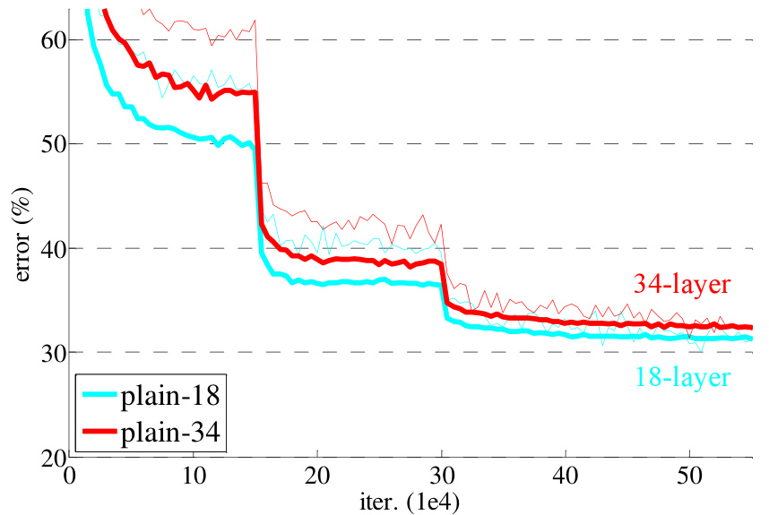
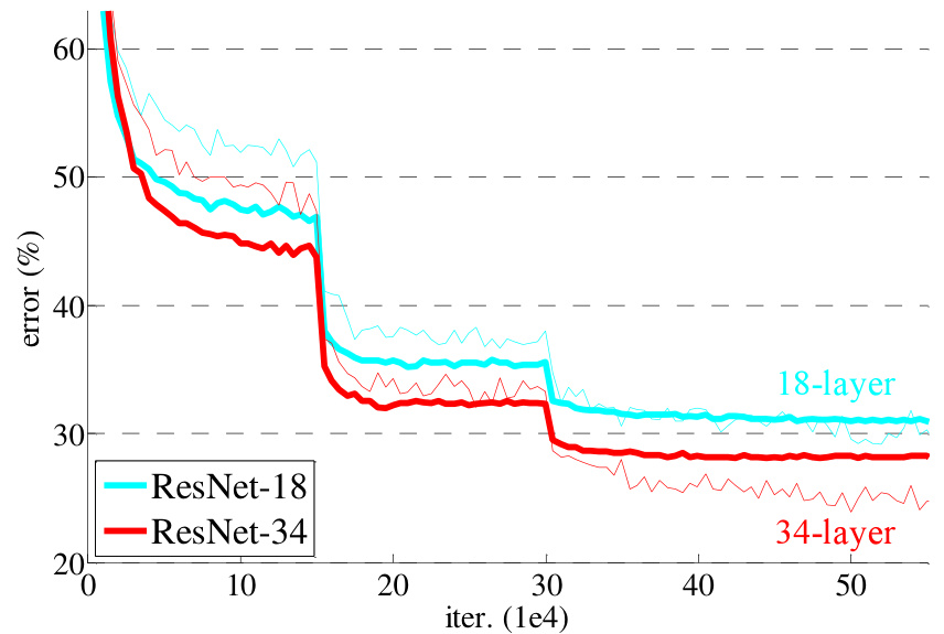
The 34-layer plain net has higher validation error than the 18-layer plain net, 28.54% against 27.94% top-1. With residual learning the situation is reversed: ResNet-34 reaches 25.03%, better than ResNet-18 by 2.8%, and exhibits considerably lower training error. Comparing the three shortcut options in the paper’s Table 3, A gives 25.03% top-1, B gives 24.52% and C — all shortcuts projections — gives 24.19%. The small differences among A/B/C indicate that projection shortcuts are not essential for addressing the degradation problem, so option C is not used, to keep memory and time complexity and model size down.
For deeper nets, a bottleneck building block replaces the stack of 2 layers with a stack of 3: \(1\times1\), \(3\times3\) and \(1\times1\) convolutions, where the \(1\times1\) layers are responsible for reducing and then increasing (restoring) dimensions, leaving the \(3\times3\) layer a bottleneck with smaller input/output dimensions. Both designs have similar time complexity.
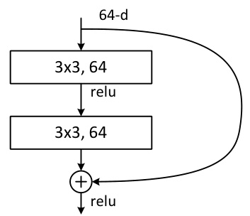
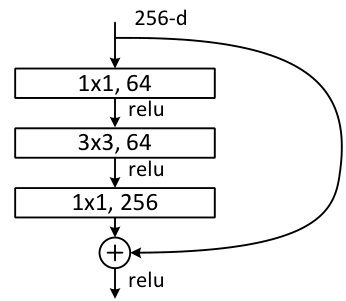
Identity shortcuts are particularly important here. If the identity shortcut is replaced with projection, the time complexity and model size are doubled, because the shortcut is connected to the two high-dimensional ends.
Replacing each 2-layer block in the 34-layer net with the 3-layer bottleneck gives ResNet-50 at 3.8 billion FLOPs; ResNet-101 and ResNet-152 follow by using more 3-layer blocks, at 7.6 and 11.3 billion FLOPs. ResNet-152 therefore still has lower complexity than VGG-16 and VGG-19 at 15.3 and 19.6 billion. Its single-model top-1 validation error is 19.38% and top-5 is 4.49%, which alone outperforms all previous ensemble results; an ensemble of six models of different depth reaches 3.57% top-5 error on the test set.
Learning outcomes
- assemble-deep-resnet-architectures Assemble ResNet-18 through ResNet-152 using basic and bottleneck blocks.
Concepts
- residual-learning inserting shortcuts into a fixed VGG-style plain baseline isolates the reformulation as the only variable in the comparison
- identity-shortcut-connection zero-padded identity, projection-on-increase, and all-projection shortcuts differ by fractions of a percent, so identity is the default
- bottleneck-building-block \(1\times1 \to 3\times3 \to 1\times1\) keeps the \(3\times3\) layer narrow, which is what makes 152 layers cheaper than VGG-19
- degradation-problem it is present in the 34-layer plain net and absent from the 50/101/152-layer residual nets
How deep can we go
The CIFAR-10 study is the controlled experiment. The architecture is deliberately simple: inputs are \(32\times32\) images with the per-pixel mean subtracted; the first layer is a \(3\times3\) convolution; then \(6n\) layers with \(3\times3\) convolutions on feature maps of sizes \(\{32, 16, 8\}\) respectively, with \(2n\) layers for each feature map size and filter counts \(\{16, 32, 64\}\); subsampling is by convolutions with a stride of 2; the network ends with global average pooling, a 10-way fully connected layer and softmax. There are \(6n{+}2\) stacked weighted layers. Shortcuts are connected to the pairs of \(3\times3\) layers, \(3n\) shortcuts in total, and identity shortcuts (option A) are used in all cases, so the residual models have exactly the same depth, width and number of parameters as the plain counterparts.
Training uses weight decay 0.0001, momentum 0.9, batch normalisation, no dropout, mini-batch 128 on two GPUs, learning rate 0.1 divided by 10 at 32k and 48k iterations, terminating at 64k, determined on a 45k/5k train/validation split. Augmentation is 4 pixels padded on each side with a \(32\times32\) crop sampled from the padded image or its horizontal flip.
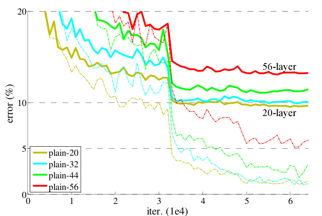
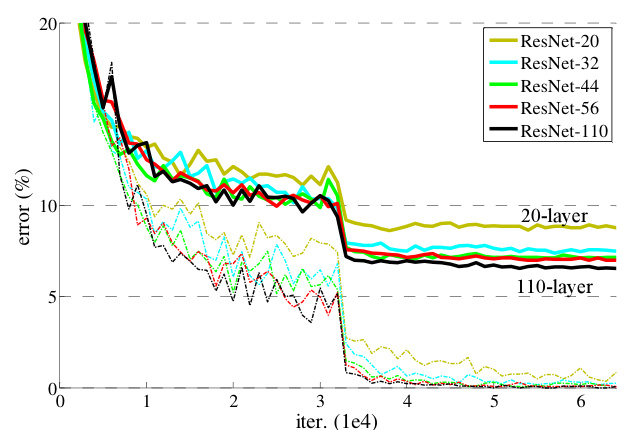
With \(n = \{3, 5, 7, 9\}\), giving 20, 32, 44 and 56 layers, the deep plain nets suffer from increased depth and exhibit higher training error as they get deeper — the same phenomenon as on ImageNet and on MNIST, which suggests that such an optimisation difficulty is a fundamental problem. The ResNets instead improve: 8.75%, 7.51%, 7.17% and 6.97% test error at those four depths, and 6.43% for ResNet-110 at 1.7M parameters. For \(n = 18\), giving 110 layers, an initial learning rate of 0.1 is slightly too large to start converging, so 0.01 is used to warm up training until the training error is below 80% (about 400 iterations), after which 0.1 resumes.
ResNet-110’s 6.43% is the “best” of five runs; the mean over runs is \(6.61 \pm 0.16\%\).
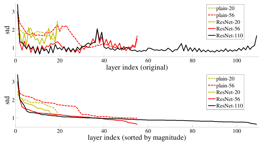
The layer-response analysis is the paper’s evidence about why. Figure 7 plots the standard deviations of the outputs of each \(3\times3\) layer, after batch normalisation and before the other nonlinearity. ResNets have generally smaller responses than their plain counterparts, which supports the motivation that the residual functions might be generally closer to zero than the non-residual functions. Response magnitudes also decrease from ResNet-20 to ResNet-56 to ResNet-110: when there are more layers, an individual layer of a ResNet tends to modify the signal less.
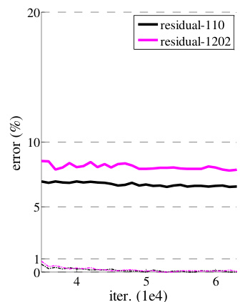
Pushing to \(n = 200\) gives a 1202-layer network. It shows no optimisation difficulty, achieving training error below 0.1%, and its test error is still fairly good at 7.93%. But that is worse than ResNet-110, although both have similar training error. The authors attribute the gap to overfitting: the 1202-layer network may be unnecessarily large for this small dataset, and no maxout or dropout is used, regularisation being imposed only via the deep and thin architecture by design. This is a different failure from degradation, and the distinction is exactly the one the first section drew — degradation shows up in training error, overfitting does not.
The same representations transfer. With Faster R-CNN as the detection method, replacing VGG-16 with ResNet-101 raises PASCAL VOC 2007 test mAP from 73.2% to 76.4% and VOC 2012 from 70.4% to 73.8%. On COCO validation, mAP@.5 rises from 41.5% to 48.4% and mAP@[.5, .95] from 21.2% to 27.2% — a 6.0 point increase on COCO’s standard metric, a 28% relative improvement, due solely to the learned representations. For ImageNet localisation, a per-class region proposal network with an RoI-centric R-CNN gives 10.6% top-5 localisation error for a single ResNet-101 model, and an ensemble reaches 9.0% on the test set, a 64% relative reduction of error against the ILSVRC 2014 result.
Learning outcomes
- analyze-depth-empirically Read the empirical evidence that residual networks gain accuracy from depth, and see where it stops.
- diagnose-the-degradation-problem Diagnose the degradation problem and distinguish it from overfitting and from vanishing gradients.
Concepts
- residual-learning layer-response standard deviations shrink with depth, which is direct evidence that the learned residual functions stay near zero
- identity-shortcut-connection option A across every pair of \(3\times3\) layers gives residual and plain nets identical depth, width and parameter count
- degradation-problem plain nets degrade from 20 to 56 layers while ResNets improve to 110, and the 1202-layer failure is overfitting rather than degradation
Densely connected blocks
Huang, Gao, et al. “Densely connected convolutional networks” (CVPR 2017) starts from the same observation about short paths and changes the combination rule. A traditional convolutional network connects the output of the \(\ell^{th}\) layer as input to the \((\ell+1)^{th}\) layer, giving the transition \(x_\ell = H_\ell(x_{\ell-1})\); a residual net adds a skip connection that bypasses the nonlinear transformations with an identity function,
\[x_\ell = H_\ell(x_{\ell-1}) + x_{\ell-1}. \tag{1}\]
An advantage of that form is that the gradient can flow directly through the identity function from later layers to the earlier layers. However, the identity function and the output of \(H_\ell\) are combined by summation, which may impede the information flow in the network. Dense connectivity keeps them apart by introducing direct connections from any layer to all subsequent layers:
\[x_\ell = H_\ell([x_0, x_1, \dots, x_{\ell-1}]), \tag{2}\]
where \([x_0, x_1, \dots, x_{\ell-1}]\) refers to the concatenation of the feature maps produced in layers \(0, \dots, \ell-1\). This introduces \(\frac{L(L+1)}{2}\) connections in an \(L\)-layer network instead of just \(L\).
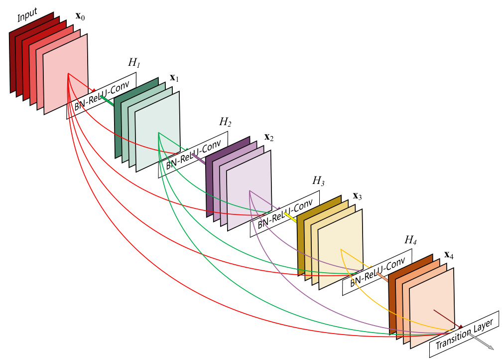
The composite function \(H_\ell(\cdot)\) is three consecutive operations: batch normalisation, a rectified linear unit, and a \(3\times3\) convolution.
Concatenation is not viable when the size of feature maps changes, and downsampling layers are essential to convolutional networks. To facilitate downsampling the network is divided into multiple densely connected dense blocks, with transition layers between them. The transition layers used in the experiments consist of a batch normalisation layer and a \(1\times1\) convolutional layer followed by a \(2\times2\) average pooling layer.

If each function \(H_\ell\) produces \(k\) feature maps, the \(\ell^{th}\) layer has \(k_0 + k \times (\ell - 1)\) input feature maps, where \(k_0\) is the number of channels in the input layer. The hyperparameter \(k\) is the growth rate, and DenseNet can have very narrow layers, for instance \(k = 12\). One explanation is that each layer has access to all the preceding feature maps in its block and therefore to the network’s “collective knowledge”. The feature maps can be viewed as the global state of the network; each layer adds \(k\) feature maps of its own to this state, and the growth rate regulates how much new information each layer contributes. The global state, once written, can be accessed from everywhere within the network, and there is no need to replicate it from layer to layer.
Two devices keep the channel count in check.
Bottleneck layers, giving DenseNet-B.
Although each layer only produces \(k\) output feature maps, it typically has many more inputs. A \(1\times1\) convolution is introduced as a bottleneck layer before each \(3\times3\) convolution, making \(H_\ell\) the sequence BN-ReLU-Conv(\(1\times1\))-BN-ReLU-Conv(\(3\times3\)), with each \(1\times1\) convolution producing \(4k\) feature maps.
Compression, giving DenseNet-C.
If a dense block contains \(m\) feature maps, the following transition layer generates \(\lfloor \theta m \rfloor\) output feature maps, where \(0 < \theta \le 1\) is the compression factor. The experiments set \(\theta = 0.5\). When both are used the model is DenseNet-BC.
For CIFAR the network has three dense blocks with an equal number of layers each, feature map sizes \(32\times32\), \(16\times16\) and \(8\times8\), and an initial convolution with 16 output channels — or twice the growth rate for DenseNet-BC. For ImageNet, four dense blocks operate on \(224\times224\) inputs with \(k = 32\) and an initial convolution of \(2k\) filters of size \(7\times7\) with stride 2.
Learning outcomes
- build-densely-connected-blocks Build a dense block where every layer receives the concatenated features of all preceding layers.
Concepts
- dense-connectivity layer \(\ell\) reads the concatenation of all preceding feature maps, so the identity signal and the new features are never merged into one tensor
- growth-rate each layer adds exactly \(k\) feature maps to a shared global state, which is why \(k = 12\) suffices
- transition-layers concatenation requires matching spatial size, so downsampling is confined to a batch normalisation, \(1\times1\) convolution and \(2\times2\) average pooling between blocks
- densenet-bc a \(1\times1\) bottleneck producing \(4k\) maps before each \(3\times3\) convolution, and transition outputs compressed by \(\theta = 0.5\)
Feature reuse and implicit supervision
Superficially, DenseNets are quite similar to ResNets: Eqn. (2) differs from Eqn. (1) only in that the inputs to \(H_\ell\) are concatenated instead of summed. The consequences of that modification, however, are substantial, and the paper’s discussion gives three of them.
Model compactness. As a direct consequence of the input concatenation, the feature maps learned by any DenseNet layer can be accessed by all subsequent layers. This encourages feature reuse throughout the network and leads to more compact models.
Implicit deep supervision. Individual layers receive additional supervision from the loss function through the shorter connections. The benefit of deep supervision was shown in deeply-supervised nets, which have classifiers attached to every hidden layer. DenseNets perform a similar deep supervision in an implicit fashion: a single classifier on top of the network provides direct supervision to all layers through at most two or three transition layers. The loss function and gradient are substantially less complicated, as the same loss function is shared between all layers.
Regularisation. On the datasets without data augmentation, the improvements over prior work are pronounced. On CIFAR-10 the improvement is a 29% relative reduction in error, from 7.33% to 5.19%; on CIFAR-100 the reduction is around 30%, from 28.20% to 19.64%.
Training is SGD, with batch size 64 for 300 epochs on CIFAR and 40 on SVHN, and batch size 256 for 90 epochs on ImageNet. The learning rate is 0.1, divided by 10 at 50% and 75% of the total epochs on CIFAR and SVHN, and at epochs 30 and 60 on ImageNet. Weight decay is \(10^{-4}\) with Nesterov momentum of 0.9 without dampening; for the three datasets without data augmentation a dropout layer with rate 0.2 is added after each convolutional layer except the first.
The numbers behind compactness are these. DenseNet-BC with \(L = 190\) and \(k = 40\) reaches 3.46% error on CIFAR-10+ and 17.18% on CIFAR-100+. DenseNet-BC with \(L = 100\) and \(k = 12\) achieves 4.51% on C10+ and 22.27% on C100+ with 0.8M parameters, comparable to the 1001-layer pre-activation ResNet’s 4.62% and 22.71% at 10.2M parameters — a 90% reduction. Capacity still helps where parameters are available: on C10+ the error drops from 5.24% to 4.10% and then 3.74% as parameters grow from 1.0M through 7.0M to 27.2M. The 250-layer DenseNet-BC does not improve on its shorter counterpart, which the authors explain by the task being relatively easy and extremely deep models overfitting.
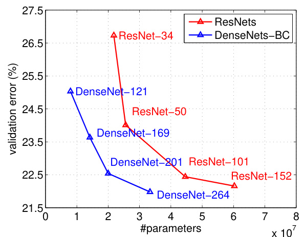
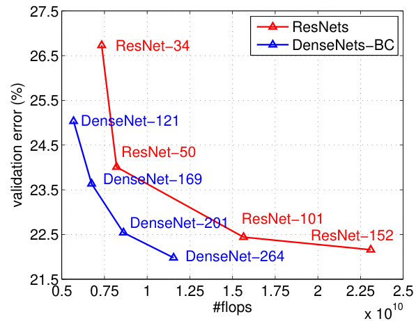
On ImageNet, DenseNet-201 with 20M parameters yields similar validation error to a 101-layer ResNet with more than 40M parameters, and a DenseNet requiring as much computation as a ResNet-50 performs on par with a ResNet-101 which requires twice as much computation. The hyperparameter settings used were optimised for ResNet, not for DenseNet.
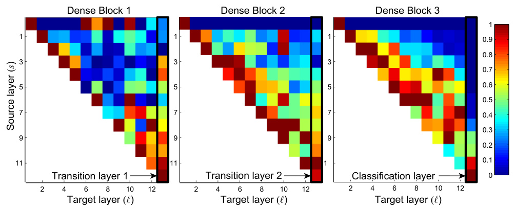
The heat map is the evidence for feature reuse. A DenseNet with \(L = 40\) and \(k = 12\) is trained on C10+, and for each convolutional layer \(\ell\) within a block the average absolute weight assigned to connections with layer \(s\) is computed; the colour of pixel \((s, \ell)\) encodes that average \(L_1\) norm, normalised by the number of input feature maps. A red dot at \((\ell, s)\) indicates that layer \(\ell\) makes on average strong use of feature maps produced \(s\) layers before. Four observations follow.
- All layers spread their weights over many inputs within the same block, so features extracted by very early layers are indeed directly used by deep layers throughout the same dense block.
- The weights of the transition layers also spread across all layers within the preceding dense block, indicating information flow from the first to the last layers of the DenseNet through few indirections.
- Layers within the second and third dense block consistently assign the least weight to the outputs of the transition layer, indicating that the transition layer outputs many redundant features with low weight on average — which is why DenseNet-BC compresses exactly those outputs.
- The final classification layer also uses weights across the entire dense block, but with a concentration toward final feature maps, suggesting some more high-level features are produced late in the network.
Learning outcomes
- explain-feature-reuse-and-implicit-supervision Explain dense connectivity’s effects: feature reuse, implicit deep supervision, and regularization.
- build-densely-connected-blocks Build a dense block where every layer receives the concatenated features of all preceding layers.
Concepts
- feature-reuse weight heat maps show deep layers drawing on feature maps produced many layers earlier, so nothing has to be re-derived
- implicit-deep-supervision one classifier supervises every layer through at most two or three transition layers, with a single shared loss
- densenet-bc 0.8M parameters match a 1001-layer ResNet’s 10.2M on CIFAR-10+, and the compression it applies targets the redundant transition outputs the heat map exposes
- growth-rate raising \(k\) from 12 to 24 buys accuracy on augmented CIFAR while narrow layers remain the reason the models are small
- transition-layers on ImageNet four dense blocks are separated by transitions that downsample \(224\times224\) inputs
SqueezeNet and the Fire module
Iandola, Forrest N., et al. “SqueezeNet: AlexNet-level accuracy with 50x fewer parameters and <0.5MB model size” (arXiv 2016) fixes the accuracy and minimises the parameters. Three engineering reasons are given for wanting that.
More efficient distributed training.
Communication among servers is the limiting factor to the scalability of distributed training, and for distributed data-parallel training the communication overhead is directly proportional to the number of parameters in the model.
Less overhead when exporting new models to clients.
For autonomous driving, companies such as Tesla periodically copy new models from their servers to customers’ cars, an over-the-air update. With AlexNet, this would require 240MB of communication from the server to the car.
Feasible FPGA and embedded deployment.
FPGAs often have less than 10MB of on-chip memory and no off-chip memory or storage. A sufficiently small model could be stored directly on the FPGA instead of being bottlenecked by memory bandwidth, while video frames stream through the FPGA in real time.
Three design strategies follow.
- Strategy 1. Replace \(3\times3\) filters with \(1\times1\) filters. Given a budget of a certain number of convolution filters, the majority are made \(1\times1\), since a \(1\times1\) filter has 9× fewer parameters than a \(3\times3\) filter.
- Strategy 2. Decrease the number of input channels to \(3\times3\) filters. For a layer comprised entirely of \(3\times3\) filters, the total quantity of parameters is (number of input channels) × (number of filters) × \((3 \times 3)\). So it is important not only to decrease the number of \(3\times3\) filters but also to decrease the number of input channels to them, which is done using squeeze layers.
- Strategy 3. Downsample late in the network so that convolution layers have large activation maps. If early layers have large strides, then most layers will have small activation maps; if most layers have a stride of 1 and the strides greater than 1 are concentrated toward the end, then many layers will have large activation maps. Large activation maps due to delayed downsampling can lead to higher classification accuracy, with all else held equal.
Strategies 1 and 2 decrease the quantity of parameters while attempting to preserve accuracy; strategy 3 is about maximising accuracy on a limited budget of parameters.
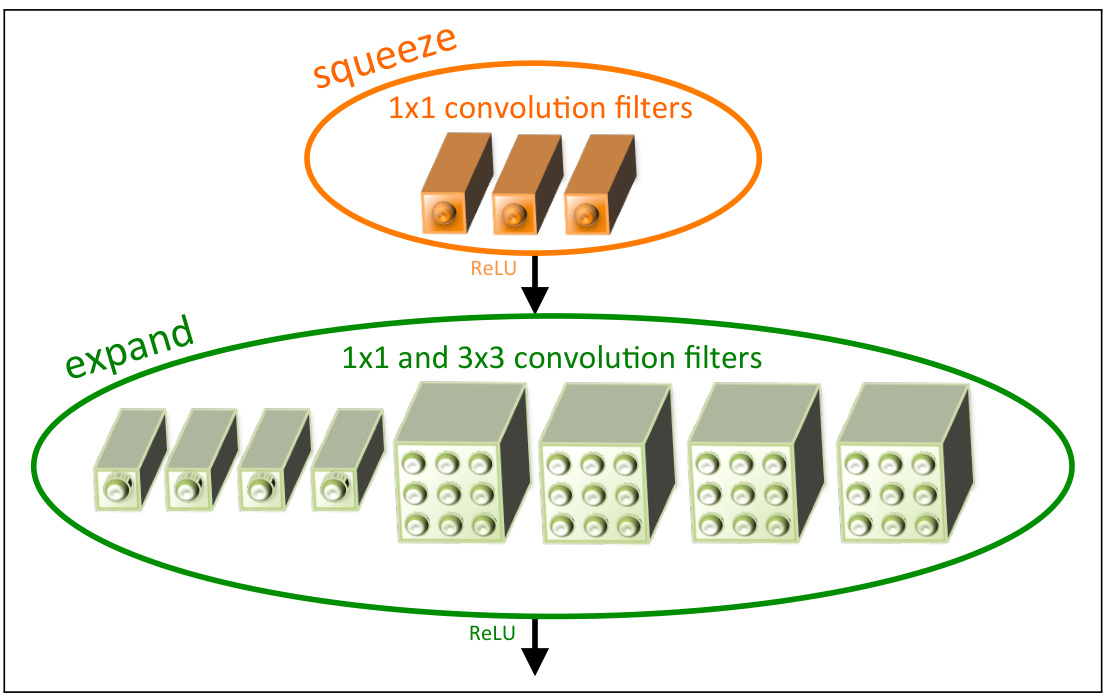
A Fire module is comprised of a squeeze convolution layer, which has only \(1\times1\) filters, feeding into an expand layer that has a mix of \(1\times1\) and \(3\times3\) convolution filters. Three tunable dimensions are exposed: \(s_{1\times1}\), the number of filters in the squeeze layer; \(e_{1\times1}\), the number of \(1\times1\) filters in the expand layer; and \(e_{3\times3}\), the number of \(3\times3\) filters in the expand layer. When Fire modules are used, \(s_{1\times1}\) is set to be less than \((e_{1\times1} + e_{3\times3})\), so the squeeze layer helps to limit the number of input channels to the \(3\times3\) filters, as per strategy 2.
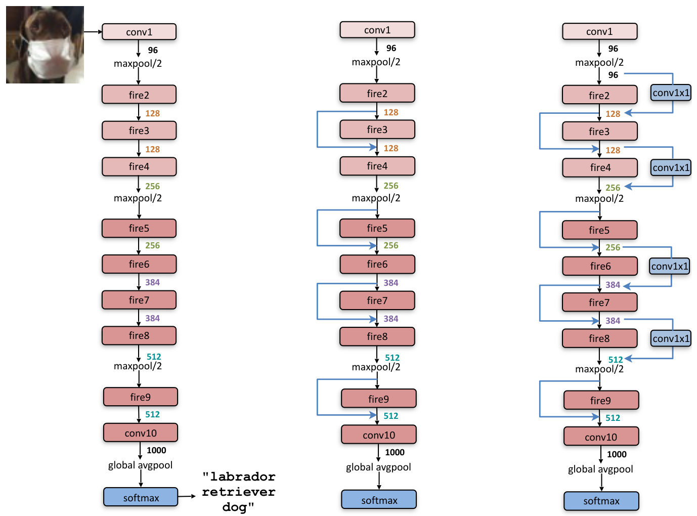
SqueezeNet begins with a standalone convolution layer conv1, followed by 8 Fire modules fire2–fire9, ending with a final convolution layer conv10. The number of filters per Fire module is gradually increased from the beginning to the end of the network. Max-pooling with a stride of 2 is performed after layers conv1, fire4, fire8 and conv10; these relatively late placements of pooling are per strategy 3. The architectural table gives conv1 as \(7\times7/2\) with 96 filters and conv10 as \(1\times1\) with 1000 filters, followed by avgpool10, for 1,248,424 parameters in total before pruning. Further details: a 1-pixel border of zero-padding is added to the input of \(3\times3\) filters of expand modules so that the \(1\times1\) and \(3\times3\) outputs have the same height and width; ReLU is applied to activations from squeeze and expand layers; dropout with a ratio of 50% is applied after the fire9 module; there are no fully connected layers, a choice inspired by Network-in-Network; and the learning rate begins at 0.04 and decreases linearly throughout training.
Against the baseline bvlc_alexnet at 240MB with 57.2% top-1 and 80.3% top-5 accuracy, uncompressed 32-bit SqueezeNet occupies 4.8MB — a 50× reduction — at 57.5% top-1 and 80.3% top-5. Applying Deep Compression with 8-bit quantisation and 33% sparsity yields a 0.66MB model, 363× smaller, at the same accuracy; with 6-bit quantisation, 0.47MB, 510× smaller. Even uncompressed, SqueezeNet is 1.4× smaller than the best result the model-compression literature had achieved on AlexNet, and the compression result answers the standing question of whether small models are amenable to compression.
Learning outcomes
- design-under-a-parameter-budget Design a CNN under a hard parameter budget using squeeze-and-expand modules.
Concepts
- squeezenet eight Fire modules between two standalone convolutions, with global average pooling and no fully connected layers, reach AlexNet accuracy at 4.8MB
- fire-module the squeeze-then-expand pair with \(s_{1\times1} < e_{1\times1} + e_{3\times3}\) enforces the input-channel strategy inside every block
- squeeze-layer \(1\times1\) filters cut the channel count reaching the \(3\times3\) filters, whose parameters scale as input channels times filters times nine
- expand-layer parallel \(1\times1\) and \(3\times3\) filters, concatenated along the channel axis, with 1-pixel padding aligning their spatial sizes
- delayed-downsampling pooling after
conv1,fire4,fire8andconv10keeps activation maps large, which raises accuracy at no parameter cost
Exploring the design space
The paper’s second contribution is method. CNN microarchitecture is the particular organisation and dimensions of the individual modules — the filter sizes within an Inception module, say. CNN macroarchitecture is the system-level organisation of multiple modules into an end-to-end architecture, which includes depth and the routing of connections across layers. Both are design spaces. Prior work on design space exploration has focused on automated approaches — Bayesian optimisation, simulated annealing, randomised search, genetic algorithms — each of which produces an architecture that beats a representative baseline, but makes no attempt to provide intuition about the shape of the design space. The alternative taken here is to refactor the network so that principled A/B comparisons can be run.
SqueezeNet has 8 Fire modules with a total of 24 dimensional hyperparameters. Rather than tune those independently, five higher-level metaparameters control the dimensions of all Fire modules in a network.
- \(base_e\) — the number of expand filters in the first Fire module.
- \(incr_e\) — the increment applied to the expand filters after every \(freq\) Fire modules, so that for Fire module \(i\) the number of expand filters is \(e_i = base_e + \left(incr_e \times \left\lfloor \frac{i}{freq} \right\rfloor \right)\).
- \(pct_{3\times3}\) — the percentage of expand filters that are \(3\times3\), shared over all Fire modules, so \(e_{i,3\times3} = e_i \times pct_{3\times3}\) and \(e_{i,1\times1} = e_i \times (1 - pct_{3\times3})\).
- \(SR\) — the squeeze ratio, shared by all Fire modules, setting \(s_{i,1\times1} = SR \times e_i\).
SqueezeNet itself is one architecture generated from this set: \(base_e = 128\), \(incr_e = 128\), \(pct_{3\times3} = 0.5\), \(freq = 2\) and \(SR = 0.125\). The name follows from the last of these — the squeeze layers have 0.125× the number of filters as the expand layers.
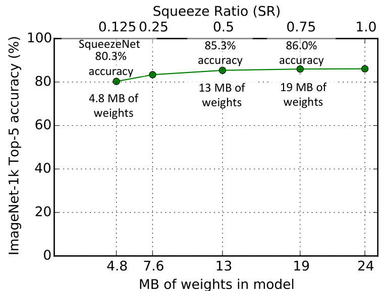
Sweeping \(SR\) over \([0.125, 1.0]\) with the other metaparameters fixed, each point on the graph an independent model trained from scratch, increasing \(SR\) beyond 0.125 raises ImageNet top-5 accuracy from 80.3% with a 4.8MB model to 86.0% with a 19MB model at \(SR = 0.75\). Accuracy plateaus at 86.0% there, and setting \(SR = 1.0\) further increases model size to 24MB without improving accuracy.
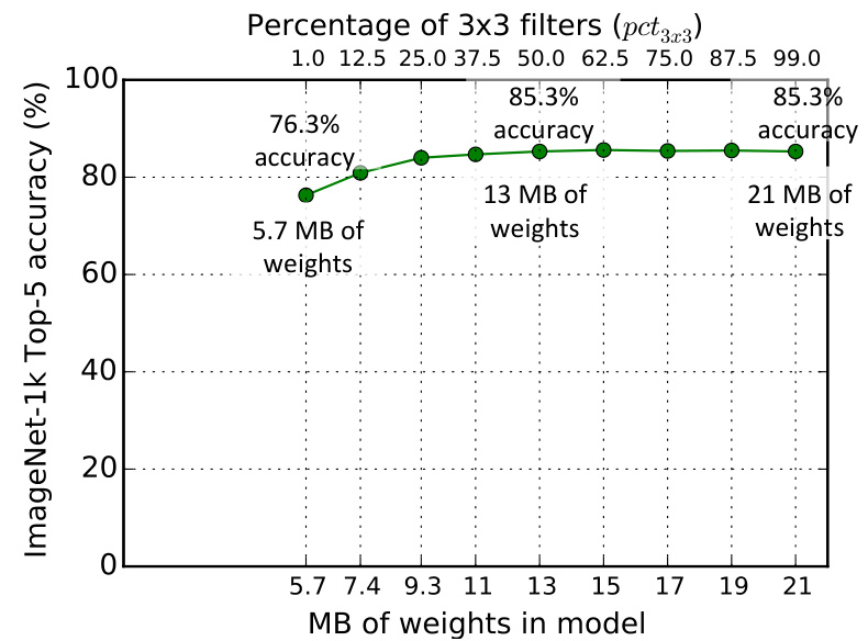
Sweeping \(pct_{3\times3}\) from 1% to 99% with \(base_e = incr_e = 128\), \(freq = 2\) and \(SR = 0.500\) turns the knob from “mostly \(1\times1\)” to “mostly \(3\times3\)”. Top-5 accuracy plateaus at 85.6% using 50% \(3\times3\) filters, and further increasing the percentage of \(3\times3\) filters leads to a larger model size but provides no improvement in accuracy on ImageNet. Both sweeps have a knee, and locating the knee is the point of running them.
At the macroarchitecture level, three variants are compared. Vanilla SqueezeNet; SqueezeNet with simple bypass connections between some Fire modules; and SqueezeNet with complex bypass connections between the remaining ones. The simple bypass architecture adds bypass connections around Fire modules 3, 5, 7 and 9, requiring these modules to learn a residual function between input and output. As in ResNet, to implement a bypass connection around Fire3, the input to Fire4 is set equal to the output of Fire2 plus the output of Fire3, where \(+\) is elementwise addition. In the straightforward case the number of input channels and the number of output channels has to be the same, so only half of the Fire modules can have simple bypass connections. When that requirement cannot be met, a complex bypass is used: a bypass that includes a \(1\times1\) convolution layer with the number of filters set equal to the number of output channels required. Complex bypass connections add extra parameters to the model, while simple bypass connections do not.
Simple bypass yields 60.4% top-1 and 82.5% top-5 accuracy at 4.8MB, against vanilla SqueezeNet’s 57.5% and 80.3% at the same size — an increase of 2.9 percentage points in top-1 and 2.2 in top-5 without increasing model size. Complex bypass gives 58.8% and 82.0% at 7.7MB, and so is beaten by the parameter-free variant. Beyond changing the regularisation, the authors’ reading is representational: with \(SR = 0.125\) every squeeze layer has 8× fewer output channels than the accompanying expand layer, and due to this severe dimensionality reduction a limited amount of information can pass through squeeze layers; adding bypass connections opens avenues for information to flow around the squeeze layers.
Learning outcomes
- explore-an-architecture-design-space Explore a CNN design space through metaparameters rather than one-off architectures.
- build-residual-blocks Build residual blocks with identity shortcuts and justify the reformulation.
Concepts
- squeeze-ratio \(SR = s_{1\times1}/(e_{1\times1}+e_{3\times3})\) raises accuracy up to 0.75 and buys only size beyond it
- fire-module four metaparameters generate all 24 filter dimensions of the eight modules, which is what makes a sweep affordable
- expand-layer the \(1\times1\) against \(3\times3\) split inside the expand layer settles at half and half
- bypass-connections-in-squeezenet elementwise addition around Fire modules 3, 5, 7 and 9 adds 2.9 points of top-1 accuracy at no parameter cost, and relieves the squeeze layers’ bottleneck
- squeezenet the released architecture is one point in this space, at \(SR = 0.125\) and \(pct_{3\times3} = 0.5\)
Depthwise separable convolutions
Howard, Andrew G., et al. “MobileNets: Efficient convolutional neural networks for mobile vision applications” (arXiv 2017) optimises primarily for latency rather than size, and gets there by restructuring the convolution operation itself.
A standard convolutional layer takes a \(D_F \times D_F \times M\) feature map \(\mathbf{F}\) and produces a \(D_F \times D_F \times N\) feature map \(\mathbf{G}\), parameterised by a kernel \(\mathbf{K}\) of size \(D_K \times D_K \times M \times N\). Assuming stride one and padding, the output is
\[\mathbf{G}_{k,l,n} = \sum_{i,j,m} \mathbf{K}_{i,j,m,n} \cdot \mathbf{F}_{k+i-1, l+j-1, m}, \tag{1}\]
at a computational cost of
\[D_K \cdot D_K \cdot M \cdot N \cdot D_F \cdot D_F. \tag{2}\]
The cost depends multiplicatively on the number of input channels \(M\), the number of output channels \(N\), the kernel size \(D_K \times D_K\), and the feature map size \(D_F \times D_F\). A standard convolution both filters and combines inputs into a new set of outputs in one step. The factorisation splits it into two layers, a separate layer for filtering and a separate layer for combining.
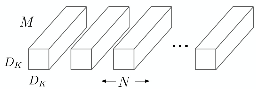
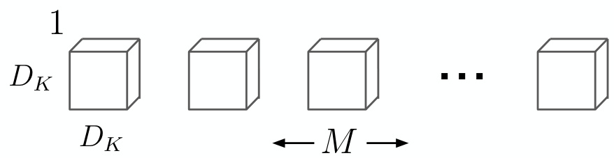
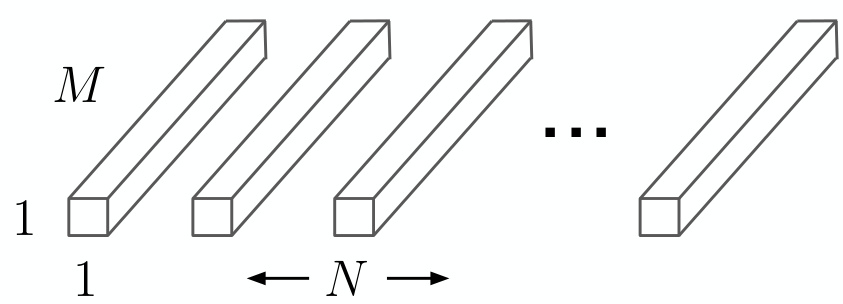
A depthwise convolution with one filter per input channel is written
\[\hat{\mathbf{G}}_{k,l,m} = \sum_{i,j} \hat{\mathbf{K}}_{i,j,m} \cdot \mathbf{F}_{k+i-1, l+j-1, m}, \tag{3}\]
where \(\hat{\mathbf{K}}\) has size \(D_K \times D_K \times M\) and the \(m\)th filter is applied to the \(m\)th channel of \(\mathbf{F}\). Its cost is \(D_K \cdot D_K \cdot M \cdot D_F \cdot D_F\). Depthwise convolution is extremely efficient relative to standard convolution, but it only filters input channels; it does not combine them to create new features. An additional layer that computes a linear combination of the output of depthwise convolution via a \(1\times1\) pointwise convolution is needed in order to generate these new features. The two together cost
\[D_K \cdot D_K \cdot M \cdot D_F \cdot D_F + M \cdot N \cdot D_F \cdot D_F, \tag{5}\]
and dividing by Eqn. (2) gives the reduction
\[\frac{D_K \cdot D_K \cdot M \cdot D_F \cdot D_F + M \cdot N \cdot D_F \cdot D_F}{D_K \cdot D_K \cdot M \cdot N \cdot D_F \cdot D_F} = \frac{1}{N} + \frac{1}{D_K^2}.\]
MobileNet uses \(3\times3\) depthwise separable convolutions, which use between 8 and 9 times less computation than standard convolutions at only a small reduction in accuracy. Further factorisation in the spatial dimension does not save much additional computation, as very little computation is spent in depthwise convolutions.
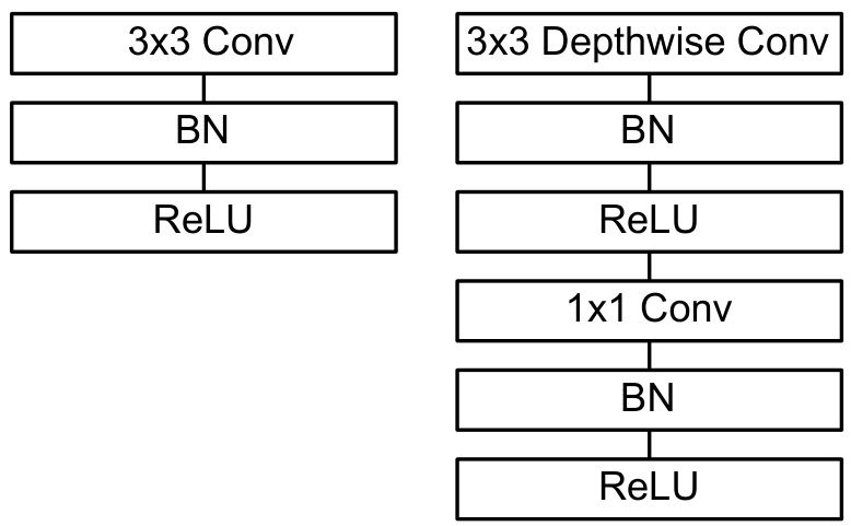
The MobileNet architecture is built on these blocks except for the first layer, which is a full convolution. All layers are followed by a batch normalisation and a ReLU nonlinearity, with the exception of the final fully connected layer, which has no nonlinearity and feeds into a softmax. Downsampling is handled with strided convolution in the depthwise convolutions as well as in the first layer, and a final average pooling reduces the spatial resolution to 1 before the fully connected layer. Counting depthwise and pointwise convolutions as separate layers, MobileNet has 28 layers.
Small multiply-add counts are not sufficient on their own; the operations also have to be efficiently implementable. Unstructured sparse matrix operations are not typically faster than dense matrix operations until a very high level of sparsity. MobileNet puts nearly all of the computation into dense \(1\times1\) convolutions: 94.86% of the multiply-adds and 74.59% of the parameters. General convolutions are often implemented by a general matrix multiply (GEMM) but require an initial reordering in memory called im2col in order to map to a GEMM; \(1\times1\) convolutions do not require this reordering and can be implemented directly with GEMM, one of the most optimised numerical linear algebra algorithms. Nearly all of the remaining parameters — 24.33% — are in the fully connected layer.
Training uses RMSprop with asynchronous gradient descent in TensorFlow. Contrary to training large models, less regularisation and data augmentation are used, because small models have less trouble with overfitting: no side heads or label smoothing, and the amount of image distortion is reduced by limiting the size of small crops. Very little or no weight decay is put on the depthwise filters, since there are so few parameters in them.
The ablation is honest about the cost. A full-convolution MobileNet reaches 71.7% ImageNet accuracy with 4866M multiply-adds and 29.3M parameters; the depthwise separable version reaches 70.6% with 569M multiply-adds and 4.2M parameters. One point of accuracy buys roughly 8.5× the computation and 7× the parameters.
Learning outcomes
- use-depthwise-separable-convolutions Factor a standard convolution into depthwise and pointwise stages and compute the saving.
Concepts
- depthwise-separable-convolution filtering and combining are split into two layers, cutting cost to \(\frac{1}{N} + \frac{1}{D_K^2}\) of a standard convolution, which is 8 to 9 times less for \(3\times3\) kernels
- depthwise-convolution one \(D_K \times D_K\) filter per input channel, with no channel mixing, so it cannot generate new features on its own
- pointwise-convolution \(1\times1\) convolutions form the linear combinations across channels and map directly to GEMM without
im2colreordering - mobilenet-architecture 28 layers of depthwise and pointwise convolutions, each followed by batch normalisation and ReLU, with strided depthwise convolutions for downsampling
Width, resolution, and choosing an operating point
One architecture is not one model. Although the base MobileNet architecture is already small and low latency, many times a specific use case or application may require the model to be smaller and faster still. Two multipliers turn the architecture into a family.
The role of the width multiplier \(\alpha\) is to thin a network uniformly at each layer. For a given layer and width multiplier \(\alpha\), the number of input channels \(M\) becomes \(\alpha M\) and the number of output channels \(N\) becomes \(\alpha N\). The computational cost of a depthwise separable convolution with width multiplier is
\[D_K \cdot D_K \cdot \alpha M \cdot D_F \cdot D_F + \alpha M \cdot \alpha N \cdot D_F \cdot D_F, \tag{6}\]
where \(\alpha \in (0, 1]\) with typical settings of 1, 0.75, 0.5 and 0.25. It has the effect of reducing computational cost and the number of parameters quadratically by roughly \(\alpha^2\). The width multiplier defines a new reduced structure that needs to be trained from scratch — it is not a post-hoc shrinking of a trained model.
The second hyperparameter is the resolution multiplier \(\rho\), applied to the input image so that the internal representation of every subsequent layer is reduced by the same multiplier. In practice \(\rho\) is set implicitly by setting the input resolution, which is 224, 192, 160 or 128. With both multipliers the cost of the core layers is
\[D_K \cdot D_K \cdot \alpha M \cdot \rho D_F \cdot \rho D_F + \alpha M \cdot \alpha N \cdot \rho D_F \cdot \rho D_F, \tag{7}\]
so \(\rho\) has the effect of reducing computational cost by \(\rho^2\), and leaves the parameter count untouched.
The paper’s worked example takes a typical internal layer with \(D_K = 3\), \(M = 512\), \(N = 512\), \(D_F = 14\), and applies the reductions cumulatively.
| Layer or modification | Million mult-adds | Million parameters |
|---|---|---|
| Convolution | 462 | 2.36 |
| Depthwise separable convolution | 52.3 | 0.27 |
| \(\alpha = 0.75\) | 29.6 | 0.15 |
| \(\rho = 0.714\) | 15.1 | 0.15 |
Accuracy drops off smoothly as \(\alpha\) falls — 70.6%, 68.4%, 63.7% and 50.6% for \(\alpha \in \{1, 0.75, 0.5, 0.25\}\) at resolution 224 — until the architecture is made too small at \(\alpha = 0.25\). Reducing resolution behaves similarly: 70.6%, 69.1%, 67.2% and 64.4% at 224, 192, 160 and 128 with \(\alpha = 1\), at 569M, 418M, 290M and 186M multiply-adds and an unchanged 4.2M parameters.
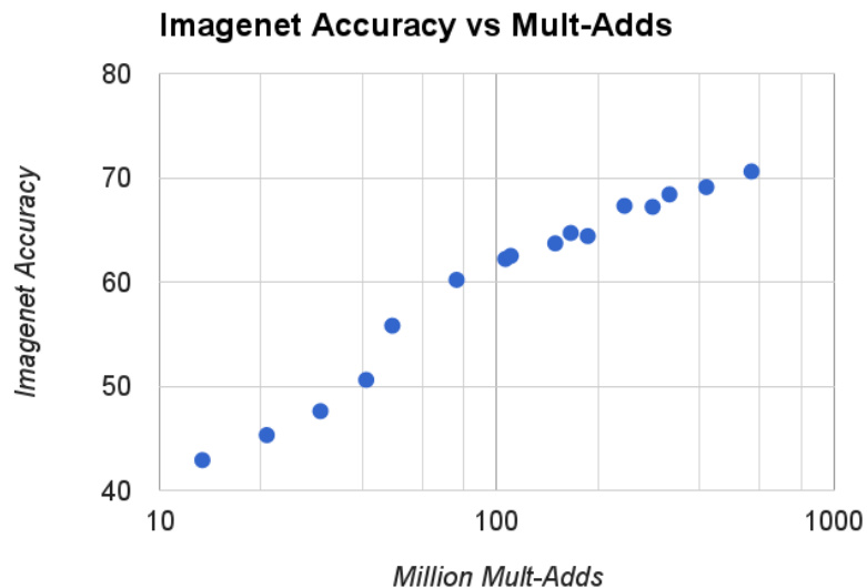
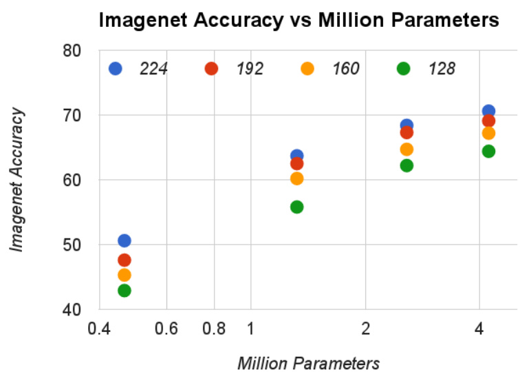
Given a budget, the choice between a thinner network and a shallower one is settled empirically. Making MobileNet shallower removes the 5 layers of separable filters with feature size \(14 \times 14 \times 512\). At similar computation and number of parameters, the 0.75 MobileNet reaches 68.4% with 325M multiply-adds and 2.6M parameters while the shallow MobileNet reaches 65.3% with 307M multiply-adds and 2.9M parameters. Making MobileNets thinner is 3% better than making them shallower, so depth is what should be preserved and width is the knob to turn.
Against the architectures of the previous unit, 1.0 MobileNet-224 at 70.6% accuracy, 569M multiply-adds and 4.2M parameters is nearly as accurate as VGG16 at 71.5% while being 32 times smaller and 27 times less compute intensive, and it is more accurate than GoogleNet at 69.8% while being smaller and using more than 2.5 times less computation. At the other end of the range, 0.50 MobileNet-160 at 60.2% accuracy, 76M multiply-adds and 1.32M parameters is 4% better than AlexNet while being 45 times smaller and using 9.4 times less computation, and 4% better than SqueezeNet at about the same size and 22 times less computation.
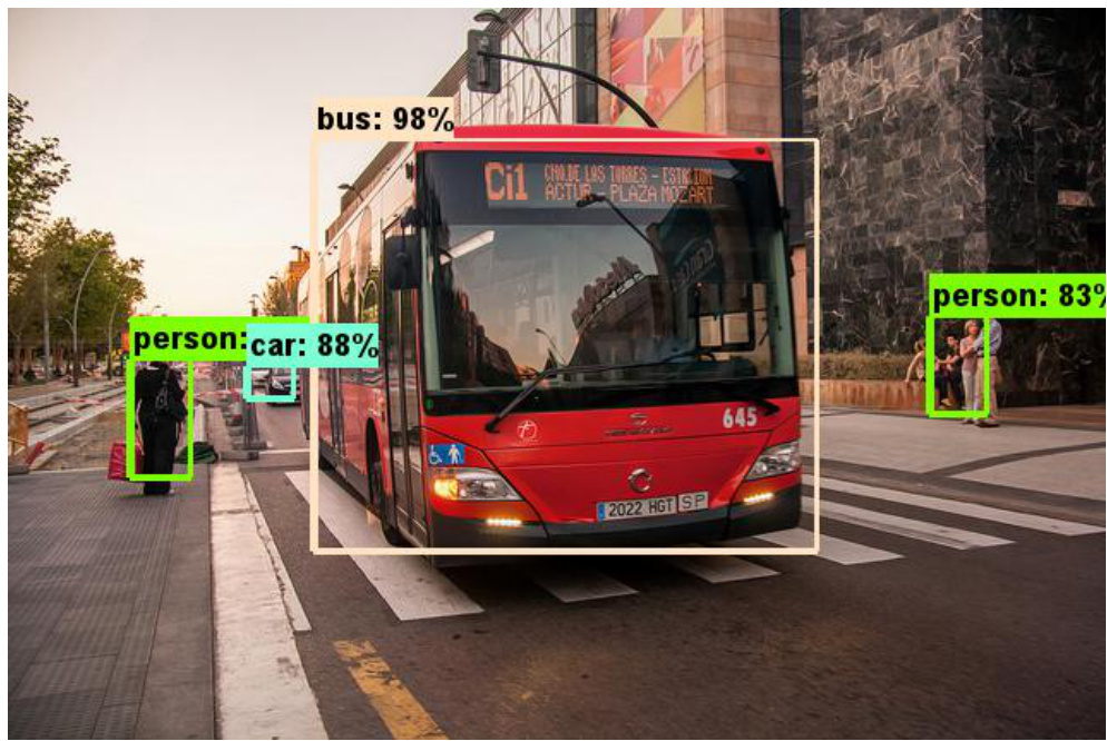
The same backbone is then substituted into several systems. On Stanford Dogs, 1.0 MobileNet-224 reaches 83.3% top-1 with 569M multiply-adds and 3.3M parameters against Inception V3’s 84.0% with 5000M and 23.2M. In PlaNet, the MobileNet version has 13 million parameters — 3 million for the body and 10 million for the final layer — and 0.58 billion multiply-adds against Inception V3’s 52 million parameters and 5.74 billion multiply-adds, and delivers 79.3% continent-scale and 11.4% street-scale localisation against 77.6% and 11.0%. A face attribute classifier of 75M parameters and 1600M multiply-adds distilled into 1.0 MobileNet-224 gives 88.7% mean average precision against the in-house baseline’s 86.9%, and 0.25 MobileNet-128 gives 86.4% at 15M multiply-adds, about 1% of the baseline’s computation. Under SSD 300 on COCO, MobileNet reaches 19.3% mAP with 1.2B multiply-adds and 6.8M parameters, against Inception V2’s 22.0% with 3.8B and 13.7M; under Faster-RCNN 600, 19.8% with 30.5B against VGG’s 25.7% with 149.6B. FaceNet embeddings distilled into 1.0 MobileNet-160 give 79.4% accuracy at a \(10^{-4}\) false accept rate with 286M multiply-adds against FaceNet’s 83% with 1600M.
Learning outcomes
- tune-width-and-resolution-multipliers Trade accuracy for latency and size with the width multiplier \(\alpha\) and resolution multiplier \(\rho\).
Concepts
- width-multiplier \(\alpha\) thins every layer, cutting cost and parameters by roughly \(\alpha^2\), and thinning beats removing layers by 3% at matched computation
- resolution-multiplier \(\rho\) shrinks the input and every internal feature map, cutting multiply-adds by \(\rho^2\) and leaving the parameter count unchanged
- depthwise-separable-convolution both multipliers enter the cost equation of the separable block, so the reductions compose
- mobilenet-architecture the same body serves classification, fine-grained recognition, geolocalisation, distilled attribute and embedding models, and SSD and Faster R-CNN detection
Key ideas
Key ideas
Degradation is an optimisation failure, and it is diagnosed on training error.
A constructed solution — a copy of a shallower net plus identity layers — always exists and is never worse, so a solver that cannot find it is the problem.
The identity shortcut is free, and that is what makes the evidence clean.
Plain and residual networks of the same depth, width and parameter count differ only by an element-wise addition, so the accuracy difference cannot be attributed to capacity.
Bottleneck blocks made depth cheaper rather than more expensive.
ResNet-152 needs 11.3 billion FLOPs, below VGG-19’s 19.6 billion, because the \(3\times3\) layer inside each block operates on reduced channel dimensions.
Concatenation and addition are not the same combination rule.
Summing merges the identity signal with the new features; concatenating keeps them distinct, which lets a dense layer contribute only \(k = 12\) new maps and read everything earlier.
Direct paths to the loss supply supervision structurally.
Every DenseNet layer sits within two or three transition layers of the single classifier, obtaining what auxiliary classifiers were added to provide.
A parameter budget is met by attacking the \(3\times3\) convolution from both sides.
Replace most \(3\times3\) filters with \(1\times1\), and squeeze the input channels of the ones that remain, since parameters scale as input channels times filters times nine.
Metaparameters turn architecture design into a sweep with a knee.
Accuracy rises with \(SR\) to 0.75 and with \(pct_{3\times3}\) to 50%, and past those points additional megabytes buy nothing.
Factoring the convolution is a different lever from pruning it.
A depthwise stage plus a pointwise stage costs \(\frac{1}{N} + \frac{1}{D_K^2}\) of a standard convolution, and because \(1\times1\) convolutions map straight to GEMM the arithmetic saving is realised as latency.
Two multipliers span an operating curve, and depth is what to keep.
\(\alpha\) cuts cost by \(\alpha^2\) and \(\rho\) by \(\rho^2\); at matched computation a thinner MobileNet is 3% more accurate than a shallower one.
Shortcut connections appear in all four papers.
Residual sums, dense concatenation, and SqueezeNet’s simple bypass are the same structural idea reached from a depth motive and from an efficiency motive.
These backbones are what the next unit consumes. Classification names an image; detection must also say where each object is and how many there are. R-CNN pairs bottom-up region proposals with convolutional features, Fast R-CNN shares that computation across regions through RoI pooling, and Faster R-CNN learns the proposals themselves with a region proposal network. Each is built on a classification backbone, which is why the shortcut connection that lifted ImageNet accuracy also lifted PASCAL VOC and MS COCO detection.
References
He, Kaiming, et al. “Deep residual learning for image recognition.” Proceedings of the IEEE conference on computer vision and pattern recognition. 2016.
Iandola, Forrest N., et al. “SqueezeNet: AlexNet-level accuracy with 50x fewer parameters and< 0.5 MB model size.” arXiv preprint arXiv:1602.07360 (2016).
Huang, Gao, et al. “Densely connected convolutional networks.” 2017 IEEE conference on computer vision and pattern recognition (CVPR). Ieee, 2017.
Howard, Andrew G., et al. “Mobilenets: Efficient convolutional neural networks for mobile vision applications.” arXiv preprint arXiv:1704.04861 (2017).