Residual Convolutional Networks

Computer Vision · v1.0.6

2026-09-25 22:16:38

Where we are

Where this fits

• VGG improved monotonically from 11 to 19 weight layers, but had to initialise deep configurations from a trained shallow one
• GoogLeNet attached auxiliary classifiers to intermediate layers to get gradient in
• Both are devices for training a deep network at all, not accounts of why it does not train

Depth is worth having, and it is fragile. Neither paper explains the fragility.

Two questions follow: what actually obstructs depth, and whether it can be removed rather than worked around; and the reverse question, at fixed accuracy how little a network can cost. Four papers answer these, and two tools carry over unchanged — the 1x1 convolution for channel mixing, and global average pooling in place of a fully connected head.

Outline of key topics

1. The degradation problem — a deep plain network trains worse, not better
2. Residual blocks and identity shortcuts
3. From VGG to ResNet: architectures, bottlenecks, depth
4. DenseNet: connectivity by concatenation
5. MobileNet: factoring the convolution itself

The degradation problem

Deeper trains worse

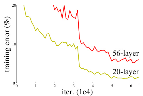
Training error: 56 layers above 20.

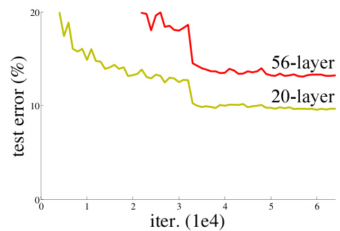
Test error: the same ordering.

A 56-layer plain network trains worse than a 20-layer one, on CIFAR-10.

Three explanations, ruled out

• Not overfitting — the gap is in training error, and overfitting fits training better, not worse
• Not vanishing gradients — batch normalization already keeps forward and backward signals healthy
• Not undertraining — three times the iterations still shows the same degradation

What remains is optimization: a solution exists, and solvers do not find it.

The construction: take a shallow network, append layers computing the identity, copy the shallow weights. This deeper network’s training error is no worse than the shallow one’s by construction. Solvers fail to find a comparably good solution, or fail to do so in feasible time — so the difficulty is in the search, not the hypothesis class.

Residual blocks and identity shortcuts

Fit the residual, not the mapping

Let \(H(x)\) be the mapping a few stacked layers must fit. Instead, fit

\[F(x) := H(x) - x\]

and recover the original as \(F(x) + x\).

If identity is close to optimal, driving \(F\) toward zero is far easier than fitting an identity through nonlinear layers.

The building block

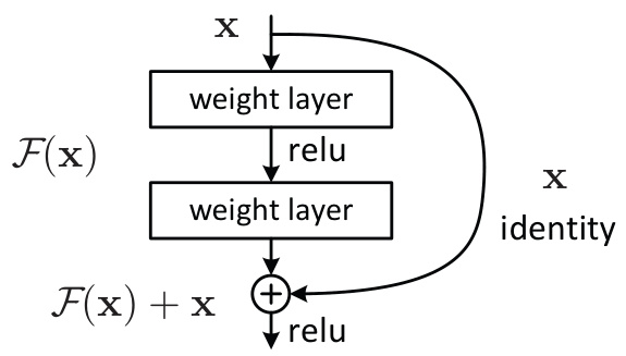
\[y = F(x, \{W_i\}) + x\]

• \(F\) is typically two weight layers with a ReLU between
• The addition is element-wise, channel by channel

No extra parameter, no meaningful extra computation.

This is what makes the experimental comparison possible: plain and residual networks of the same depth, width and parameter count differ only by the addition. A shortcut across a single layer gives no benefit – it just reparameterises a linear map. Two or three layers is the useful range.

Choosing a shortcut

Same dimensions

• Identity shortcut, no parameters

Dimensions increase

• Option A — zero-pad the extra channels, still parameter-free
• Option B — a projection \(y = F(x,\{W_i\}) + W_s x\)

Projections help slightly; identity is the default because the gain does not justify the cost.

From VGG to ResNet

The plain and residual baselines

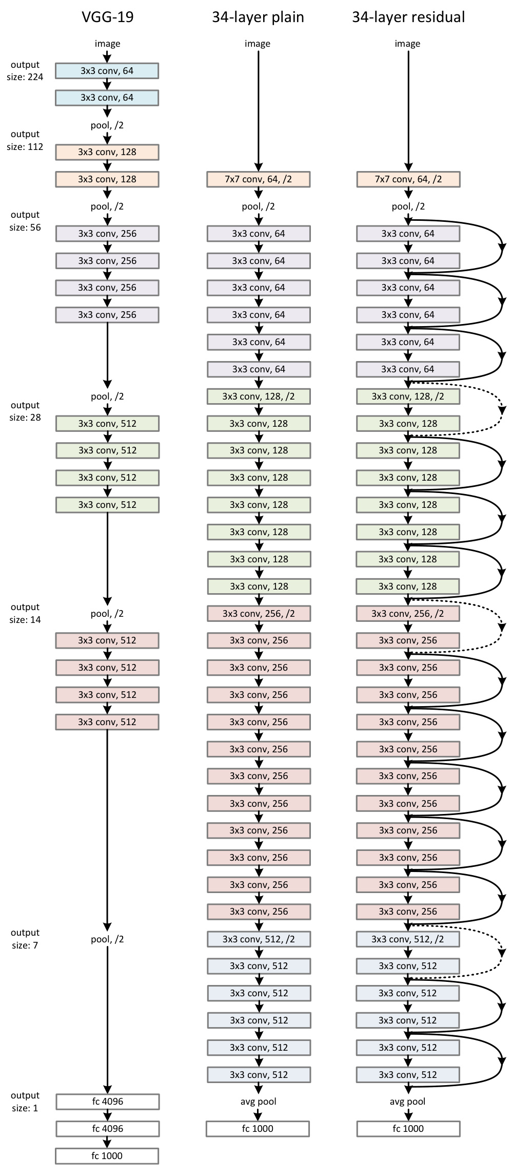
VGG-19, the 34-layer plain network, and the 34-layer residual network — shortcuts inserted every two layers, nothing else changed.

VGG-style design rules: same filter count for the same feature map size, filters double when the size halves, downsampling by stride-2 convolutions, global average pooling into the softmax. The 34-layer plain net costs 3.6 billion FLOPs, 18% of VGG-19’s 19.6 billion.

Bottleneck blocks for depth

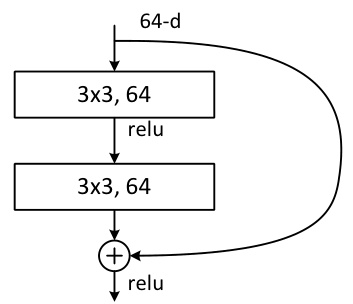
Two-layer block, ResNet-34.

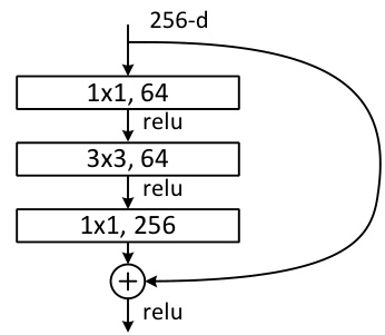
Bottleneck block, ResNet-50/101/152.

\(1\times1 \to 3\times3 \to 1\times1\): reduce, then restore.

Identity shortcuts matter most here: a projection on a bottleneck doubles its cost.

The ResNet family

Network	Layers	FLOPs	Top-5 error
VGG-19	19	19.6 B	—
ResNet-34	34	3.6 B	—
ResNet-50	50	3.8 B	—
ResNet-101	101	7.6 B	—
ResNet-152	152	11.3 B	4.49%

152 layers, at lower cost than 19. Depth became cheaper, not more expensive.

An ensemble of six models of different depth reaches 3.57% top-5 on the test set, first to outperform prior ensembles with a single-model result alone.

Plain against residual, by depth

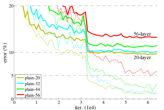
Plain nets: higher error as depth grows, 20 to 56 layers.

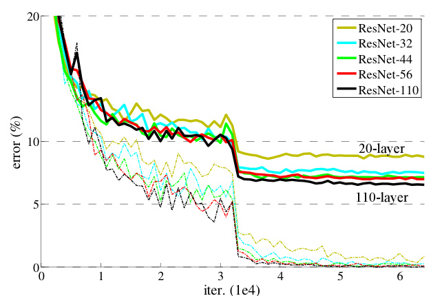
ResNets: lower error as depth grows, to 110 layers.

The crossover is the whole argument: the same depths, opposite trends.

Pushing to 1202 layers

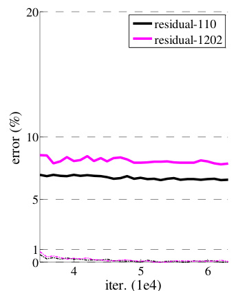
ResNet-110 against ResNet-1202.

Training error falls under 0.1% — but test error is worse than at 110. Overfitting, not degradation.

Densely connected blocks

Dense connectivity

A residual layer adds the identity back: \(x_\ell = H_\ell(x_{\ell-1}) + x_{\ell-1}\).

\[x_\ell = H_\ell([x_0, x_1, \dots, x_{\ell-1}])\]

• Every layer receives the concatenation of all preceding feature maps
• An \(L\)-layer block carries \(L(L+1)/2\) connections, not \(L\)

Concatenation keeps the identity and the new features distinct; summation merges them.

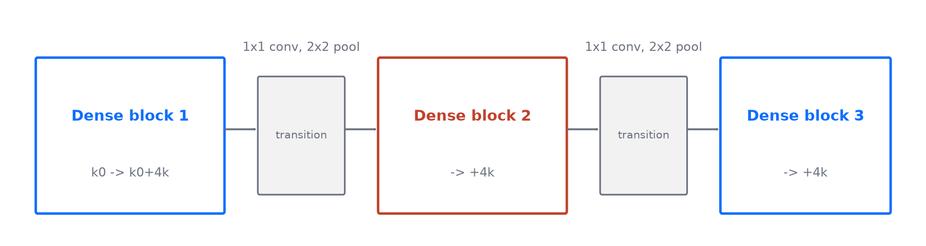
One dense block

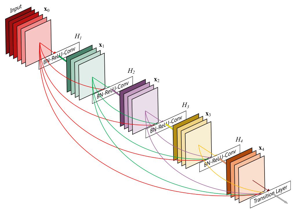
A 5-layer dense block, growth rate \(k=4\). Each layer takes every earlier feature map as input.

From blocks to a network

Transitions — batch norm, a 1x1 convolution, 2x2 average pooling — are the only place channel count is cut back.

Growth rate k as small as 12 is competitive: each layer adds only k feature maps to a shared collective state that every later layer can read, so nothing needs to be re-derived. DenseNet-B adds a 1x1 bottleneck producing 4k maps before each 3x3; DenseNet-BC also compresses transition outputs by theta = 0.5.

DenseNet against ResNet

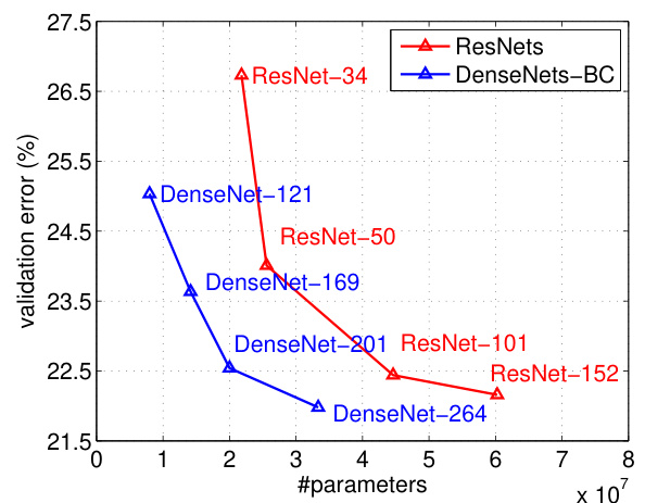
Accuracy against parameter count.

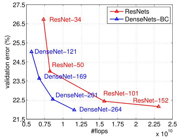
Accuracy against FLOPs.

A DenseNet at ResNet-50’s computation performs on par with ResNet-101, at half the FLOPs.

Deeper without degrading

• DenseNet-BC at 0.8M parameters matches a 1001-layer pre-activation ResNet’s 10.2M — a 90% reduction
• Every layer sits within two or three transitions of the classifier: implicit deep supervision
• Feature-reuse heat maps show deep layers drawing on feature maps from many layers earlier

Concatenation lets DenseNet go deeper than ResNet, at a fraction of the parameters.

Depth-wise separable convolutions in Mobilenet

The cost of a standard convolution

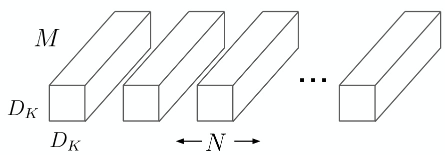
Standard filters: every output reads every input channel.

A kernel \(D_K \times D_K \times M \times N\) maps an \(M\)-channel input to an \(N\)-channel output:

\[D_K \cdot D_K \cdot M \cdot N \cdot D_F \cdot D_F\]

• One layer both filters each channel and combines channels into new ones

What if filtering and combining were two cheaper layers instead of one expensive one?

Stage one: depthwise convolution

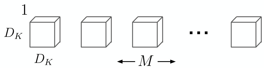
One \(D_K \times D_K\) filter per input channel.

\[\hat{\mathbf{G}}_{k,l,m} = \sum_{i,j} \hat{\mathbf{K}}_{i,j,m} \cdot \mathbf{F}_{k+i-1,\, l+j-1,\, m}\]

• \(\hat{\mathbf{K}}\) has size \(D_K \times D_K \times M\) — no \(N\) index
• The \(m\)th filter sees only the \(m\)th channel
• Cost: \(D_K \cdot D_K \cdot M \cdot D_F \cdot D_F\)

It filters each channel and cannot combine them, so it creates no new features.

Stage two: pointwise convolution

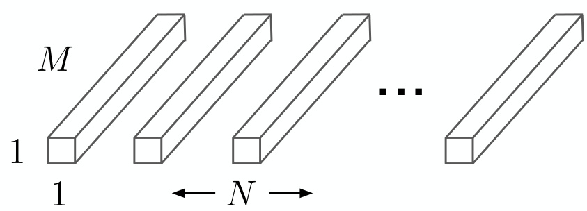
A \(1\times1\) kernel across all \(M\) channels.

\[\mathbf{G}_{k,l,n} = \sum_{m} \mathbf{K}_{m,n} \cdot \hat{\mathbf{G}}_{k,l,m}\]

• A linear combination across channels at one position
• No spatial extent: \(D_K = 1\)
• Cost: \(M \cdot N \cdot D_F \cdot D_F\)

It combines channels into the \(N\) new features the depthwise stage could not produce.

The pointwise equation is the standard convolution of equation (1) with the kernel size set to one, applied to the depthwise output rather than to the input. That is why the two stages compose into a replacement for the standard convolution rather than an approximation of a different operator.

The saving, per convolution

Depthwise costs \(D_K \cdot D_K \cdot M \cdot D_F \cdot D_F\); pointwise adds \(M \cdot N \cdot D_F \cdot D_F\). Together, against the standard convolution:

\[\frac{1}{N} + \frac{1}{D_K^2}\]

For a 3x3 kernel: 8 to 9 times less computation, at a small accuracy cost.

Further factoring the spatial dimension saves little more, since very little computation is spent in the depthwise stage to begin with.

The replacement

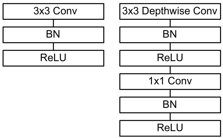
A standard convolutional layer with batch norm and ReLU (left), against the depthwise separable pair (right).

MobileNet puts nearly all computation into dense 1x1 convolutions – 94.86% of the multiply-adds – which map directly to GEMM without an im2col reordering step, so the arithmetic saving is realised as latency, not only as a smaller parameter count.

Summary

What this unit established

• Degradation is an optimization failure, diagnosed on training error
• The identity shortcut is free — no extra parameters or computation
• Bottleneck blocks: ResNet-152 costs less than VGG-19
• Concatenation is not summation: DenseNet adds only \(k\) channels per layer
• Factoring a convolution is a different lever from pruning it

Shortcut connections recur across every architecture in this unit.

Where next

These backbones are what object detection consumes.

• Classification names an image; detection must also say where and how many
• R-CNN pairs region proposals with convolutional features
• The backbone that lifted ImageNet accuracy lifts detection accuracy too

A better backbone lifts every downstream task.