Lecture notes — 2021 Clip
ver. 1.0.0, 2021_clip
ver. 1.0.0 · 2026-08-22 10:25:50
Where we are
In Chapter 18: Diffusion models we built a generative model that turns noise into an image through a learned reverse chain. We then steered that chain. Classifier guidance and classifier-free guidance both push the sampler towards a class \(c\) or towards a text prompt.
One assumption was left unexamined. Something has to map a prompt into a vector the model can condition on, and something has to compute a score between a prompt and a partially generated image. This unit builds that something.
The paper is Radford, Alec, et al. “Learning transferable visual models from natural language supervision.” International conference on machine learning. PmLR, 2021. It introduces CLIP — Contrastive Language-Image Pre-training — an image encoder and a text encoder trained jointly so that matching image-text pairs land near each other in one shared embedding space. Training uses 400 million (image, text) pairs collected from the internet and no hand-annotated labels at all.
The immediate payoff is zero-shot transfer: any set of class names becomes a classifier, with no training on the target dataset. The payoff for the next unit is that a caption can now score an image.
Learning outcomes
- natural-language-supervision Explain why raw text is a better supervision signal than a fixed set of labels.
- contrastive-objective Write the symmetric contrastive objective CLIP is trained on and explain its efficiency.
- zero-shot-classification Build a zero-shot classifier from class names, using prompt engineering and ensembling.
What you will be able to do
natural-language-supervision— Explain why raw text is a better supervision signal than a fixed set of labels.webimagetext-dataset— Describe how the 400M-pair WebImageText dataset was constructed and why its scale matters.contrastive-objective— Write the symmetric contrastive objective CLIP is trained on and explain its efficiency.architecture-and-scaling— Describe CLIP’s dual-encoder architecture and how each side is scaled.zero-shot-classification— Build a zero-shot classifier from class names, using prompt engineering and ensembling.representation-quality— Evaluate CLIP’s features with linear probes and few-shot transfer, and read the results.effective-robustness— Explain effective robustness and why zero-shot CLIP degrades less under distribution shift.limitations-and-human-baseline— Identify where CLIP fails, and compare its sample efficiency with a human’s.bias-and-impacts— Assess the biases CLIP inherits from uncurated web data and the deployment risks that follow.
What we will cover
- Natural Language Supervision — training visual models directly from unstructured web text rather than fixed, crowd-labelled categorical labels.
- WebImageText (WIT) Dataset — a web-scale dataset of 400 million image-text pairs curated using a wide query vocabulary.
- Contrastive Language-Image Pre-training (CLIP) — a multimodal framework that jointly trains an image encoder and a text encoder via a contrastive loss to predict correct image-text pairs.
- Zero-Shot Visual Transfer — classifying unseen image datasets by generating linear classifier weights from class text descriptions.
- Prompt Engineering and Ensembling — customising and ensembling natural language text templates to raise zero-shot accuracy.
- Effective Robustness — gains in out-of-distribution accuracy exceeding what in-distribution accuracy predicts.
Natural language as supervision
State-of-the-art vision systems are trained to predict a fixed set of predetermined object categories. The paper opens by naming the cost of that choice. Supervision of this restricted form limits generality and usability, because additional labelled data is needed to specify any other visual concept.
Natural language supervision means learning perception from the supervision contained in the text that already accompanies images. The authors are careful to point out that the idea is not new. Prior work described the same manoeuvre as unsupervised, self-supervised, weakly supervised and supervised in turn. What is common across that line of work is not the method but the appreciation of natural language as a training signal.
Two strengths are claimed for it.
It is much easier to scale than crowd-sourced labelling.
Annotations need not be in a “machine learning compatible format” such as the canonical 1-of-N majority vote gold label. A method that works on natural language can learn passively from the text already on the internet.
It connects the representation to language.
Most unsupervised methods “just” learn a representation. Learning from text binds that representation to words, which is what enables flexible zero-shot transfer: classifying an unseen dataset by generating classifier weights from its class names.
Why earlier attempts underperformed
The introduction surveys the record honestly. Mori et al. (1999) predicted nouns and adjectives in paired documents. Joulin et al. (2016) trained CNNs to predict words in captions. Li et al. (2017) extended this to phrase n-grams and demonstrated zero-shot transfer by scoring class names against a dictionary of learned visual n-grams.
The results were modest. Li et al. (2017) reach only 11.5% accuracy on ImageNet in a zero-shot setting — well below the 88.4% of the state of the art at the time, and even below the 50% of classic computer vision approaches.
The diagnosis is scale, not principle. Mahajan et al. (2018) and Kolesnikov et al. (2019) trained on millions to billions of images for accelerator years; VirTex, ICMLM and ConVIRT trained for accelerator days on one to two hundred thousand images. The weakly supervised middle ground also carries a second cost: those works limit their supervision to 1000 and 18291 classes respectively, and use static softmax classifiers with no mechanism for dynamic outputs.
Natural language “is able to express, and therefore supervise, a much wider set of visual concepts through its generality.” That generality is the whole argument.
Key ideas
- A closed label set bounds what a model can ever say. Text does not.
- Captions require no annotator, so supervision scales with the web rather than with a budget.
- Binding the representation to language is what makes zero-shot transfer possible at all.
- Earlier text-supervised vision failed on scale, not on the idea.
Learning outcomes
- natural-language-supervision Explain why raw text is a better supervision signal than a fixed set of labels.
Concepts
- natural-language-supervision defines natural language supervision as the foundational training signal for learning visual representations
- zero-shot-transfer explains that natural language supervision enables flexible zero-shot transfer by connecting visual representations to text
Building WebImageText
A motivation for natural language supervision is the quantity of such data available publicly. Existing datasets did not reflect that possibility, so results on them would underestimate the approach. The authors therefore built their own.
Why the existing datasets fell short
Prior work had mainly used three.
MS-COCO and Visual Genome are high quality crowd-labelled datasets, but small by modern standards — approximately 100,000 training photos each.
For comparison, other vision systems are trained on up to 3.5 billion Instagram photos.
YFCC100M, at 100 million photos, is a possible alternative, but its metadata is sparse and of varying quality.
Many images use automatically generated filenames such as
20160716_113957.JPGas titles, or contain “descriptions” of camera exposure settings. After filtering to keep only images with natural language titles or descriptions in English, the dataset shrank by a factor of 6 to only 15 million photos — approximately the size of ImageNet.
The construction
WebImageText, abbreviated WIT, is a new dataset of 400 million (image, text) pairs collected from a variety of publicly available sources on the internet. Its construction has three parts.
- A query list of 500,000 terms. The base list is all words occurring at least 100 times in the English Wikipedia. It is augmented with bi-grams of high pointwise mutual information, the names of all Wikipedia articles above a certain search volume, and finally all WordNet synsets not already present.
- Query-conditioned search. Pairs are collected whose text includes one of the 500,000 queries. Coverage is therefore broad by construction rather than by luck.
- Approximate class balancing. Up to 20,000 (image, text) pairs are included per query. A handful of very common terms cannot dominate the result.
The scale is best understood by comparison to language modelling. The resulting dataset has a similar total word count to the WebText dataset used to train GPT-2. This is language-model-scale data applied to vision.
The pairs are unfiltered and uncurated. That is exactly what makes the collection cheap, and exactly what makes the biases we examine later unavoidable. Keep the two facts attached to one another.
Learning outcomes
- webimagetext-dataset Describe how the 400M-pair WebImageText dataset was constructed and why its scale matters.
Concepts
- webimagetext-dataset details the curation, query design, and construction of the WebImageText (WIT) dataset
- natural-language-supervision demonstrates the need for web-scale datasets to harness natural language supervision effectively
The contrastive objective
Training efficiency was the criterion by which the final method was selected. The authors state the reason plainly. Mahajan et al. (2018) required 19 GPU years for their ResNeXt101-32x48d; Xie et al. (2020) required 33 TPUv3 core-years for Noisy Student EfficientNet-L2. Both systems were trained to predict only 1000 ImageNet classes. Learning an open set of visual concepts from natural language on that budget seems daunting.
Two objectives that failed to scale
The initial approach, similar to VirTex, jointly trained an image CNN and a text transformer from scratch to predict the caption of an image. It scaled badly. A 63 million parameter transformer language model — already using twice the compute of its ResNet-50 image encoder — learns to recognise ImageNet classes three times slower than a much simpler baseline that predicts a bag-of-words encoding of the same text.
Both approaches share one flaw. They try to predict the exact words of the text accompanying each image, and that is difficult given the wide variety of descriptions, comments and related text that co-occur with images.
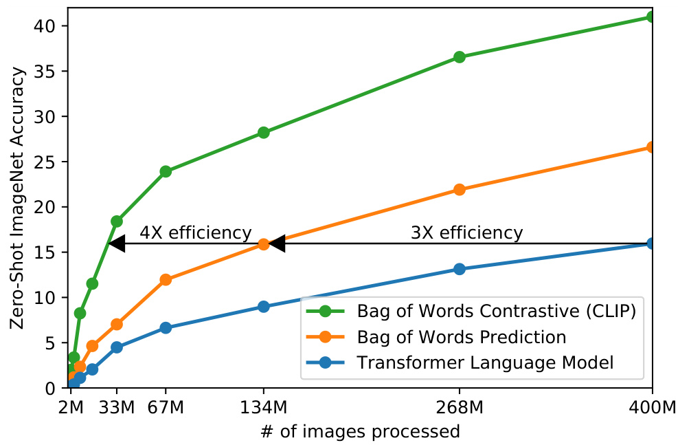
Starting from the bag-of-words baseline and swapping the predictive objective for a contrastive one gave a further 4x improvement in the rate of zero-shot transfer to ImageNet.
The task
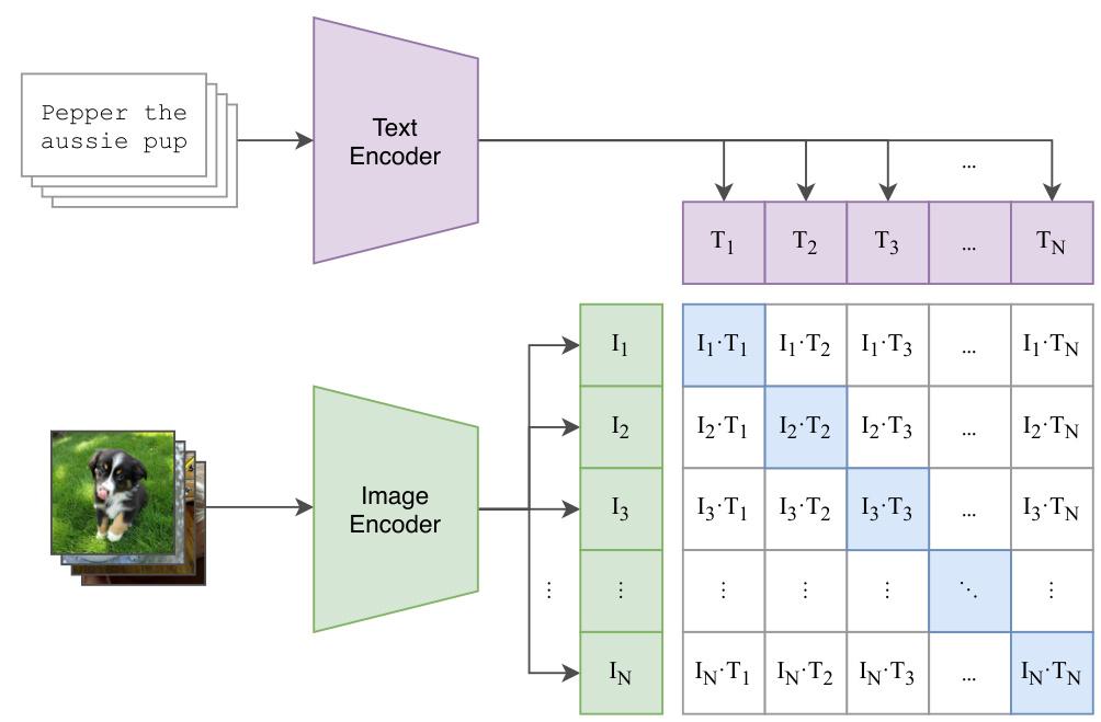
Given a batch of \(N\) (image, text) pairs, CLIP is trained to predict which of the \(N \times N\) possible pairings across the batch actually occurred. It learns a multi-modal embedding space by jointly training an image encoder and a text encoder to maximise the cosine similarity of the \(N\) real pairs while minimising the cosine similarity of the \(N^2 - N\) incorrect pairings. A symmetric cross-entropy loss is optimised over these similarity scores.
Figure 3 of the paper gives the core of an implementation.
# extract feature representations of each modality
I_f = image_encoder(I) #[n, d_i]
T_f = text_encoder(T) #[n, d_t]

# joint multimodal embedding [n, d_e]
I_e = l2_normalize(np.dot(I_f, W_i), axis=1)
T_e = l2_normalize(np.dot(T_f, W_t), axis=1)

# scaled pairwise cosine similarities [n, n]
logits = np.dot(I_e, T_e.T) * np.exp(t)

# symmetric loss function
labels = np.arange(n)
loss_i = cross_entropy_loss(logits, labels, axis=0)
loss_t = cross_entropy_loss(logits, labels, axis=1)
loss = (loss_i + loss_t)/2
Read it line by line. Each modality is encoded, projected by a learned matrix, and L2-normalised. The logits are the matrix of pairwise cosine similarities, scaled by \(\exp(t)\) where t is a learned temperature parameter. The correct labels are simply np.arange(n) — the \(i\)-th image belongs with the \(i\)-th text. Cross-entropy is taken once down the columns and once across the rows, and the two are averaged. That averaging is what makes the loss symmetric in the two modalities.
The negatives are the other members of the batch. A larger batch is therefore a harder task and a stronger signal.
This batch construction was first introduced in deep metric learning as the multi-class N-pair loss (Sohn, 2016), popularised for contrastive representation learning as the InfoNCE loss (Oord et al., 2018), and adapted to (text, image) pairs in medical imaging by Zhang et al. (2020).
Simplifications
Because the pre-training set is so large, over-fitting is not a major concern, and the recipe is simplified relative to Zhang et al. (2020).
- Both encoders are trained from scratch, with no ImageNet initialisation and no pre-trained language model.
- There is no non-linear projection between the representation and the contrastive embedding space — only a linear projection.
- A random square crop from resized images is the only data augmentation used during training.
- The temperature \(\tau\) is directly optimised during training as a log-parameterised multiplicative scalar, rather than tuned as a hyper-parameter.
Learning outcomes
- contrastive-objective Write the symmetric contrastive objective CLIP is trained on and explain its efficiency.
Concepts
- contrastive-language-image-pretraining introduces the contrastive symmetric cross-entropy objective and architecture for CLIP
- webimagetext-dataset applies the contrastive pre-training method over the WIT dataset
Encoders and scaling
Nothing above says what the two encoders are. The paper considers two families on the image side and one on the text side.
The image encoder
A modified ResNet. ResNet-50 is the base architecture. Three modifications are made: the ResNet-D improvements of He et al. (2019), the antialiased rect-2 blur pooling of Zhang (2019), and the replacement of global average pooling with an attention pooling mechanism.
The attention pooling is implemented as a single layer of transformer-style multi-head QKV attention where the query is conditioned on the global average-pooled representation of the image.
A Vision Transformer. The implementation of Dosovitskiy et al. (2020) is followed closely, with one minor modification: an additional layer normalisation on the combined patch and position embeddings before the transformer, plus a slightly different initialisation scheme.
The text encoder
The text encoder is a Transformer with the modifications of Radford et al. (2019). The base size is a 63M-parameter, 12-layer, 512-wide model with 8 attention heads. It operates on a lower-cased byte pair encoding of the text with a 49,152 vocabulary. For computational efficiency the maximum sequence length is capped at 76.
The text sequence is bracketed with [SOS] and [EOS] tokens. The activations of the highest layer at the [EOS] token are the feature representation of the text. Those activations are layer-normalised and then linearly projected into the multi-modal embedding space. Masked self-attention is used throughout, so that the encoder could later be initialised from a pre-trained language model — an option the paper leaves for future work.
The only interaction between the image and text domains in a CLIP model is a single dot product in the learned joint embedding space. Nothing is fused early. That is precisely why a classifier can be cached once and reused, and why retrieval over a large corpus is cheap.
Scaling
Previous vision research often scaled by increasing width or depth in isolation. For the ResNet image encoders CLIP adapts the approach of Tan & Le (2019), allocating additional compute across all of width, depth and resolution. Where EfficientNet tunes the ratio between those dimensions, CLIP uses the simple baseline of allocating additional compute equally to each. The text encoder is scaled in width only, proportional to the increase in ResNet width, and not scaled in depth at all — performance was found to be less sensitive to text encoder capacity.
Training
Five ResNets and three Vision Transformers were trained: ResNet-50, ResNet-101, and RN50x4, RN50x16, RN50x64 at roughly 4x, 16x and 64x the compute of a ResNet-50; and ViT-B/32, ViT-B/16, ViT-L/14.
- All models are trained for 32 epochs with the Adam optimizer, decoupled weight decay on all weights that are not gains or biases, and a cosine learning rate schedule.
- The learnable temperature \(\tau\) is initialised to the equivalent of 0.07 and clipped to prevent scaling the logits by more than 100, which was necessary to prevent training instability.
- The minibatch size is 32,768.
- Mixed precision, gradient checkpointing, half-precision Adam statistics and half-precision stochastically rounded text encoder weights were all used to save memory. Embedding similarity computation was sharded across GPUs.
- The largest ResNet, RN50x64, took 18 days on 592 V100 GPUs. The largest Vision Transformer took 12 days on 256 V100 GPUs.
- ViT-L/14 was additionally pre-trained at a higher 336 pixel resolution for one extra epoch, in the manner of FixRes. This model, ViT-L/14@336px, is what the paper means by “CLIP” unless stated otherwise.
Learning outcomes
- architecture-and-scaling Describe CLIP’s dual-encoder architecture and how each side is scaled.
Concepts
- contrastive-language-image-pretraining specifies the image and text encoder architectures used in CLIP models
Zero-shot transfer
CLIP is pre-trained to predict whether an image and a text snippet are paired. Zero-shot classification reuses that capability directly.
The construction
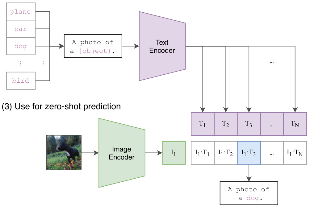
For each dataset, take the names of all the classes as the set of potential text pairings and predict the most probable (image, text) pair. Concretely: embed the image, embed the set of possible texts, compute cosine similarity, scale by the temperature \(\tau\), and normalise into a probability distribution with a softmax.
Read that prediction layer carefully. It is a multinomial logistic regression classifier with L2-normalised inputs, L2-normalised weights, no bias, and temperature scaling. Under that reading the image encoder is the vision backbone, and the text encoder is a hypernetwork that generates the weights of a linear classifier from text specifying the visual concepts the classes represent. Change the class names, get a different classifier, with no gradient steps.
The classifier is cached once it has been computed, so the cost of generating it is amortised across every prediction on the dataset.
Every step of pre-training can be viewed as optimising a randomly created proxy dataset with one example per class and 32,768 total classes, each defined by a natural language description.
The first comparison
Visual N-Grams (Li et al., 2017) is the only prior work to study zero-shot transfer to standard image classification datasets with a generically pre-trained model. Table 1 of the paper compares the two.
| aYahoo | ImageNet | SUN | |
|---|---|---|---|
| Visual N-Grams | 72.4 | 11.5 | 23.0 |
| CLIP | 98.4 | 76.2 | 58.5 |
CLIP improves ImageNet accuracy from a proof of concept 11.5% to 76.2%, matching the original ResNet-50 despite using none of its 1.28 million crowd-labelled training examples. Its top-5 accuracy is 95%, matching Inception-V4. On aYahoo it achieves a 95% reduction in errors, and on SUN it more than doubles the earlier accuracy.
The authors caution against reading this as a methods comparison. They train on a dataset 10x larger, use a vision model requiring nearly 100x more compute per prediction, and likely used over 1000x the training compute.
Prompt engineering
Class names as released are often unhelpful. Two problems recur.
- Polysemy. A bare word carries no context. ImageNet contains both construction cranes and cranes that fly. In Oxford-IIIT Pets,
boxerclearly means a breed of dog, but a text encoder without context could as easily read it as a type of athlete. - Distribution mismatch. It is relatively rare in the pre-training data for the text paired with an image to be a single word. Usually it is a full sentence.
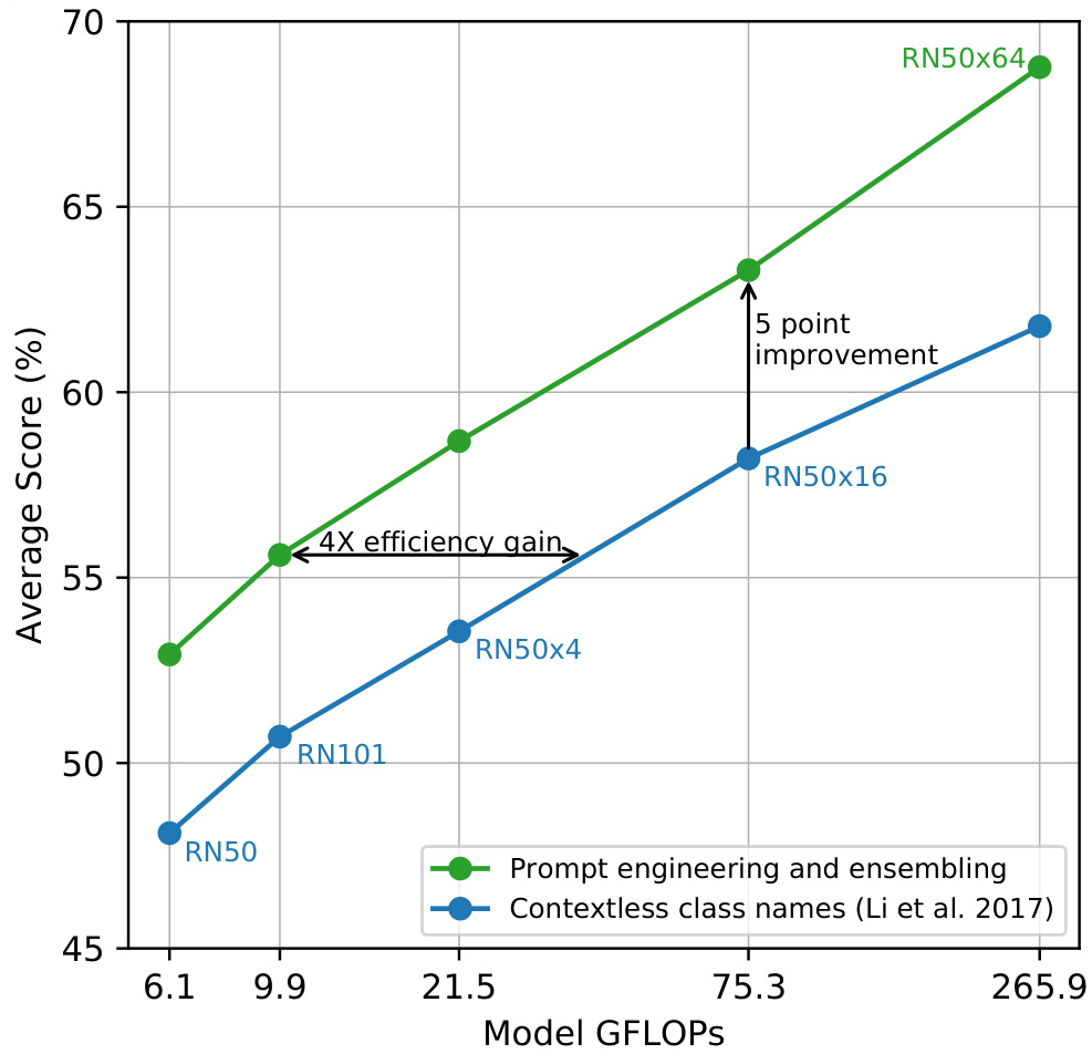
Prompt engineering addresses both. The default template "A photo of a {label}." specifies that the text is about the content of the image, and improves ImageNet accuracy by 1.3% on its own. Task-specific context helps more.
- Oxford-IIIT Pets:
"A photo of a {label}, a type of pet." - Food101: specify a type of food; FGVC Aircraft: a type of aircraft.
- Satellite datasets: variants of
"a satellite photo of a {label}." - OCR datasets: put quotes around the text or number to be recognised.
Prompt ensembling
Prompt ensembling computes several zero-shot classifiers from different context prompts — for instance 'A photo of a big {label}' and "A photo of a small {label}" — and combines them. The ensemble is constructed in embedding space, not probability space. A single set of averaged text embeddings can therefore be cached, so the ensemble costs the same as a single classifier when amortised over many predictions.
On ImageNet, 80 different context prompts are ensembled, improving performance by a further 3.5% over the single default prompt. Together, prompt engineering and ensembling improve ImageNet accuracy by almost 5%.
How good is it?
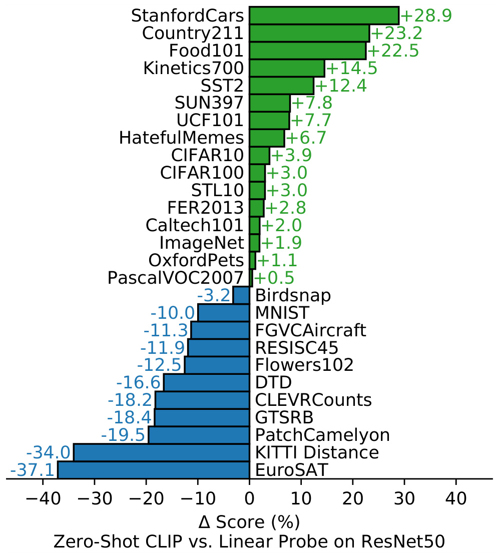
The baseline is a fully supervised, regularised logistic regression classifier fitted on the features of the canonical ResNet-50. Across a 27 dataset suite, zero-shot CLIP wins on 16 of the 27 datasets, including ImageNet.
The spread is instructive.
- On Stanford Cars and Food101 zero-shot CLIP beats the baseline by over 20%; on Flowers102 and FGVCAircraft it underperforms by over 10%. The authors attribute this to varying per-task supervision between WIT and ImageNet.
- On general object classification — ImageNet, CIFAR10/100, STL10, PascalVOC2007 — performance is similar, with a slight advantage to CLIP in all cases. On STL10 CLIP reaches 99.3%, a new state of the art without a single training example.
- On action recognition in video CLIP is much stronger: +14.5% over ResNet-50 on Kinetics700 and +7.7% on UCF101. Natural language supplies wider supervision for concepts involving verbs than ImageNet’s noun-centric labels.
- It is weak on specialised, complex or abstract tasks: satellite imagery (EuroSAT, RESISC45), lymph node tumour detection (PatchCamelyon), counting objects in synthetic scenes (CLEVRCounts), German traffic signs (GTSRB), and distance to the nearest car (KITTI Distance).
Zero-shot performance also scales. Averaging error across 39 evaluations on 36 datasets, a log-log linear trend holds across a 44x range of compute spanning five CLIP models — though individual evaluations are far noisier than the aggregate.
Key ideas
- The text encoder is a hypernetwork that writes the weights of a linear classifier from class names.
- Prompts matter because a bare label is both ambiguous and unlike a caption.
- Ensembling in embedding space is free at inference time; ensembling in probability space would not be.
- Zero-shot CLIP beats a supervised ResNet-50 linear probe on 16 of 27 datasets, and is near-random on several others.
Learning outcomes
- zero-shot-classification Build a zero-shot classifier from class names, using prompt engineering and ensembling.
Concepts
- zero-shot-transfer provides extensive empirical evaluation of CLIP’s zero-shot classification capabilities across downstream datasets
- prompt-engineering-and-ensembling demonstrates how prompt engineering and ensembling significantly boost zero-shot accuracy
- contrastive-language-image-pretraining examines zero-shot performance scaling as a function of compute across CLIP model sizes
Representation learning evaluation
“CLIP does zero-shot” and “CLIP has good features” are two different claims. They are measured differently, and this section measures the second.
Why linear probes
Two options exist: fit a linear classifier on the frozen representation, or fine-tune the model end to end. Fine-tuning outperforms linear classification on most image classification datasets, so its use would be defensible. The paper chooses linear probes anyway, for reasons worth internalising.
- Fine-tuning adapts representations to each dataset, which can compensate for and mask failures to learn general representations during pre-training. Linear classifiers, being inflexible, expose those failures.
- Linear probing is very similar to how the zero-shot classifiers are built, which makes the two directly comparable.
- Scale. Studying 66 different models on 27 different datasets requires tuning 1782 evaluations. Fine-tuning opens a much larger hyperparameter space; linear classifiers require minimal tuning and have standardised procedures.
The comparison
On the 12-dataset suite of Kornblith et al. (2019) — chosen first, to minimise selection effects — the small CLIP models do not win. ResNet-50 and ResNet-101 outperform other ResNets trained on ImageNet-1K, but underperform BiT-M models trained on ImageNet-21K and EfficientNets of similar compute.
CLIP models scale well, however. The largest ResNet, RN50x64, slightly outperforms Noisy Student EfficientNet-L2 on both overall score and compute efficiency. CLIP vision transformers are about 3x more compute efficient than CLIP ResNets. The best overall model, ViT-L/14@336px, outperforms the best existing model on this suite by an average of 2.6%.
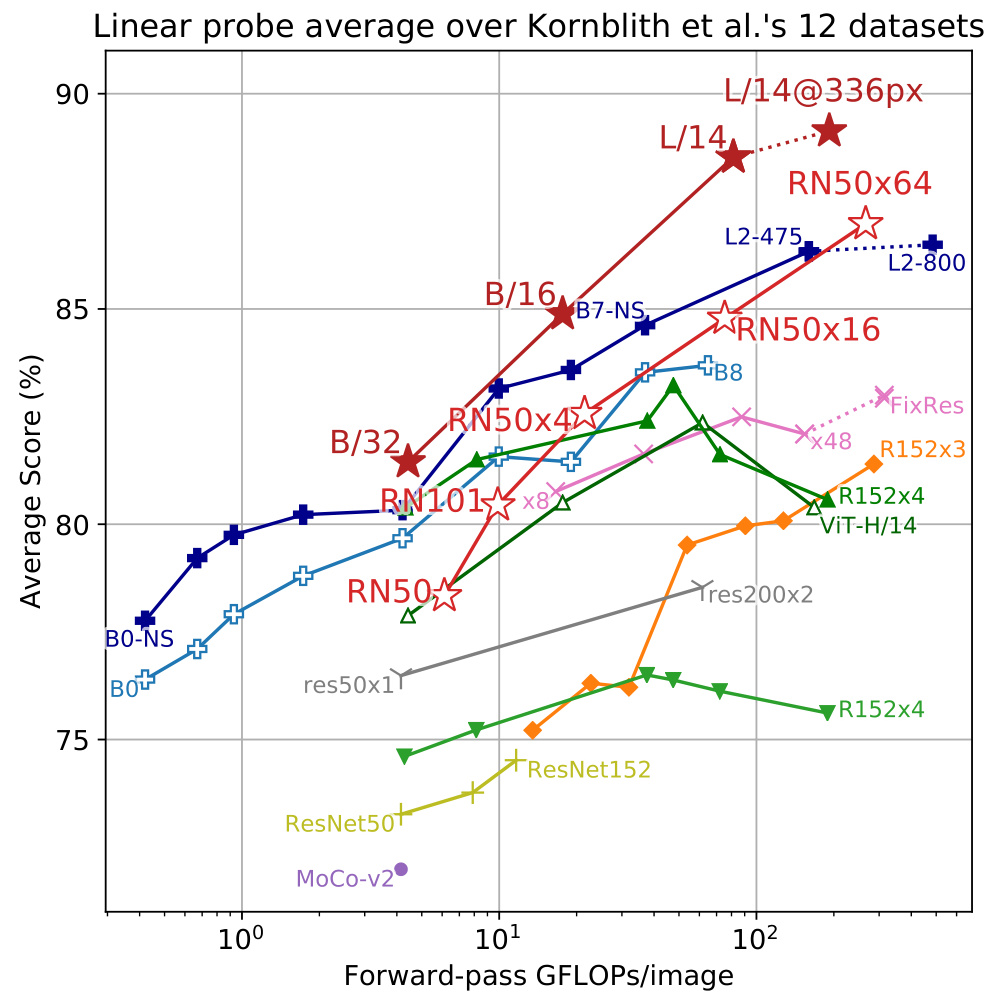
The 12-dataset suite arguably carries a selection bias towards tasks that overlap with ImageNet. CLIP learns geo-localization, OCR, facial emotion recognition and action recognition, none of which appear in it. On the broader 27-dataset suite the improvement in average score over previous systems rises from 2.6% to 5%, and all CLIP models, regardless of scale, outperform every evaluated system on compute efficiency.
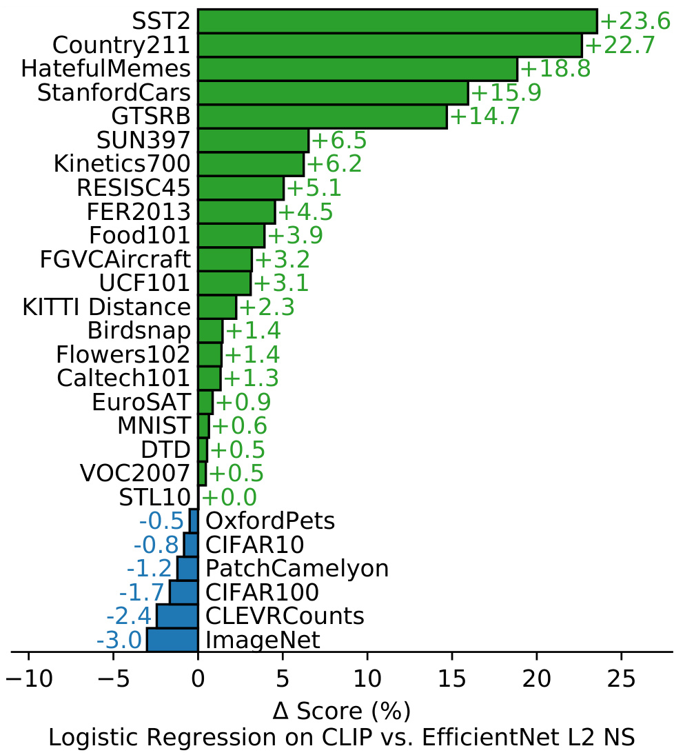
Per dataset, CLIP wins on 21 of 27. It gains most on OCR (SST2, HatefulMemes), geo-localization and scene recognition (Country211, SUN397), video activity recognition (Kinetics700, UCF101), and fine-grained car and traffic sign recognition. The 14.7% improvement on GTSRB may indicate a problem with ImageNet-1K itself, which has a single label for all traffic and street signs — narrow supervision that encourages a representation to collapse intra-class detail. The EfficientNet wins, unsurprisingly, on ImageNet, and on low-resolution datasets such as CIFAR10 and CIFAR100, likely from CLIP’s lack of scale-based augmentation.
Few-shot, and a surprise
Comparing zero-shot to few-shot is the more direct comparison, since zero-shot is few-shot’s limit. One would expect zero-shot to underperform one-shot. Instead, zero-shot CLIP matches the performance of a 4-shot logistic regression trained on the same feature space, and roughly matches the best 16-shot classifier in the suite, a BiT-M ResNet-152x2 trained on ImageNet-21K.
The explanation is that a zero-shot classifier is generated from language, so the visual concept is communicated directly. Example-based learning must infer the concept indirectly, and many hypotheses are consistent with one image, which usually contains many visual concepts at once.
Data efficiency varies widely by dataset — from under one labelled example per class to 184. Half the datasets require fewer than 5 examples per class, with a median of 5.4, but the mean is 20.8 because roughly 20% of datasets need many. On ImageNet, zero-shot CLIP matches a 16-shot linear classifier on its own features.
Zero-shot performance correlates with fully supervised linear probe performance at 0.82, but sits 10 to 25 points lower on most datasets. It approaches the supervised ceiling on only five: STL10, CIFAR10, Food101, OxfordPets and Caltech101 — all datasets where both accuracies exceed 90%.
Learning outcomes
- representation-quality Evaluate CLIP’s features with linear probes and few-shot transfer, and read the results.
Concepts
- contrastive-language-image-pretraining measures representation quality of pre-trained CLIP models using linear probes
Robustness under distribution shift
In 2015 a deep learning model was announced to exceed human performance on the ImageNet test set. Subsequent research found those models still make many simple mistakes, and new benchmarks put their performance far below both their ImageNet accuracy and human accuracy.
The common explanation is that deep learning models are exceedingly adept at finding correlations and patterns which hold across their training dataset. Many of those correlations are spurious, do not hold on other distributions, and produce large drops in performance there.
Effective robustness
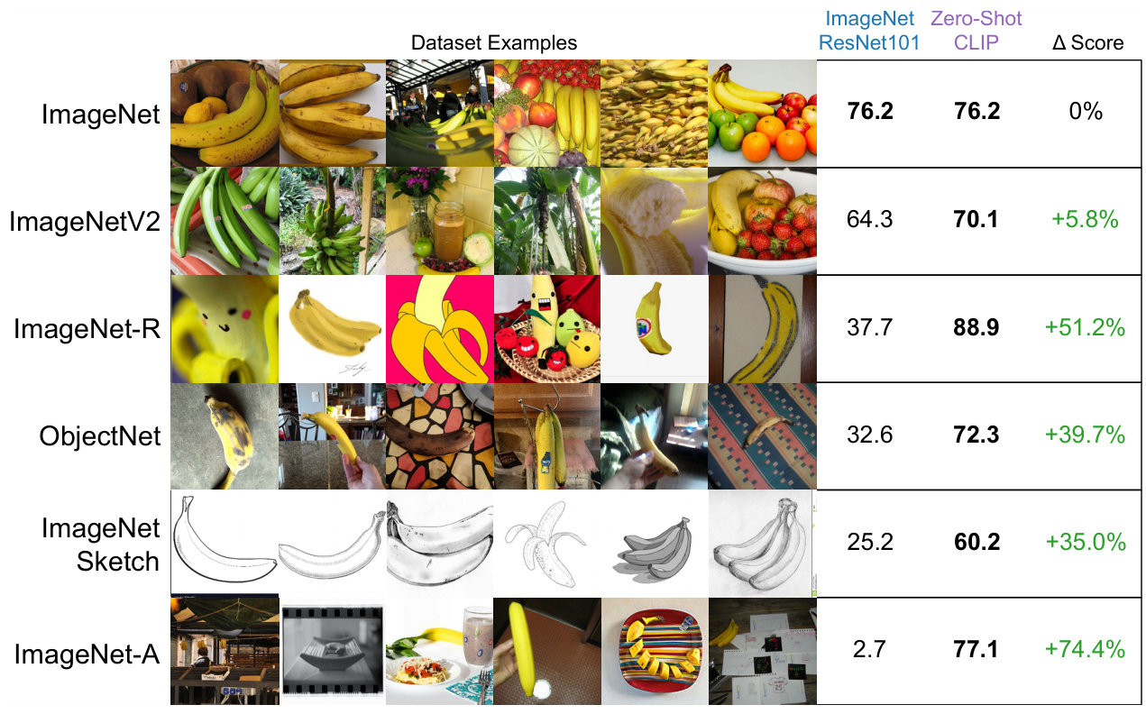
Taori et al. (2020) studied seven natural distribution shifts: ImageNetV2, ImageNet Sketch, Youtube-BB, ImageNet-Vid, ObjectNet, ImageNet Adversarial and ImageNet Rendition. These consist of novel images collected from various sources. They are deliberately distinguished from synthetic shifts such as ImageNet-C or adversarial attacks, which perturb existing images — techniques that improve the synthetic case often fail to help on the natural one.
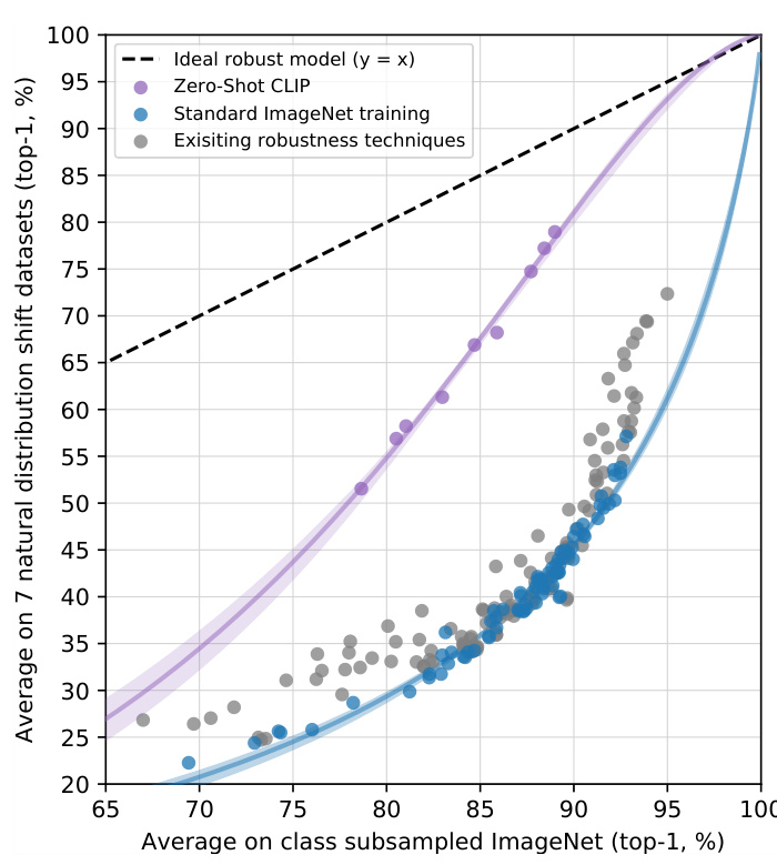
A ResNet-101 makes five times as many mistakes on these shifts as on the ImageNet validation set. But accuracy under shift increases predictably with ImageNet accuracy, and is well modelled as a linear function of logit-transformed accuracy. Every model sits close to one line.
That observation supports a distinction.
Effective robustness measures improvements in accuracy under distribution shift above what is predicted by the documented relationship between in-distribution and out-of-distribution accuracy.
Geometrically, it is the vertical distance from the line.
Relative robustness captures any improvement in out-of-distribution accuracy at all.
A model can gain relative robustness simply by being more accurate. Effective robustness is the harder claim.
CLIP’s result
Almost every model in Taori et al. (2020) was trained or fine-tuned on ImageNet. A zero-shot model should not be able to exploit correlations that hold only on a distribution it never saw. All zero-shot CLIP models improve effective robustness by a large amount and reduce the gap between ImageNet accuracy and accuracy under distribution shift by up to 75%.
The trade-off when you adapt
Fitting an L2-regularised logistic regression on CLIP features on the ImageNet training set raises ImageNet accuracy by 9.2% to 85.4%, tying the 2018 state of the art. Average accuracy under distribution shift slightly decreases.
A 9.2% gain corresponds to roughly three years of state-of-the-art progress, and it buys nothing under shift. Broken down per dataset, performance rises significantly on only one — ImageNetV2, which closely followed the original ImageNet creation process. Elsewhere it falls: 4.7% on ImageNet-R, 3.8% on ObjectNet, 2.8% on ImageNet Sketch, and 1.9% on ImageNet-A. Gains from supervised adaptation are concentrated around the ImageNet distribution.
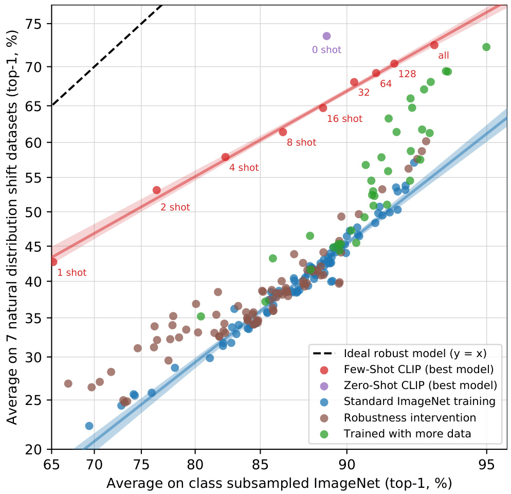
The continuum makes the trade-off explicit. Few-shot models also show higher effective robustness than existing models, but the benefit fades as more training data is added and is mostly gone for the fully supervised model. High effective robustness seems to result from minimising the amount of distribution-specific training data a model has access to — at the cost of reduced dataset-specific performance.
Because a zero-shot classifier is built from names, you can also fix mismatched taxonomies. Youtube-BB and ImageNet-Vid consist of superclasses of ImageNet, and a fixed 1000-way classifier must pool predictions — the person class is pooled from baseball player, bridegroom and scuba diver. Generating a custom zero-shot classifier per dataset improves average effective robustness by 5%.
Learning outcomes
- effective-robustness Explain effective robustness and why zero-shot CLIP degrades less under distribution shift.
Concepts
- effective-robustness analyses CLIP’s effective robustness across seven natural distribution shift datasets
- zero-shot-transfer demonstrates that zero-shot transfer minimises reliance on spurious correlations compared to supervised training
Limitations, overlap and humans
A strong headline result should be read sceptically. The paper reads its own that way, across three separate analyses.
Data overlap
With 400 million web pairs, some evaluation images may have been seen during pre-training. In a worst case a complete copy of an evaluation set could leak in and invalidate the test entirely.
One option is to remove all duplicates before training. That guarantees true hold-out performance, but requires knowing every dataset a model might ever be evaluated on. Adding a new evaluation would then demand an expensive re-train. The paper instead documents how much overlap occurs and what it does.
The procedure is worth learning as a method.
- Run a duplicate detector on each evaluation dataset. Manually inspect the nearest neighbours and set a per-dataset threshold that keeps high precision while maximising recall. This partitions the set into Overlap and Clean, with the untouched set called All.
- Compute zero-shot accuracy of CLIP RN50x64 on the three splits and report All − Clean as the main metric — the difference in accuracy attributable to contamination.
- Run a binomial significance test using accuracy on Clean as the null hypothesis, and compute 99.5% Clopper-Pearson confidence intervals as a further check.
The findings: of 35 datasets, 9 have no detected overlap at all — mostly synthetic or specialised sets such as MNIST, CLEVR and GTSRB, or sets guaranteed clean by date, such as ObjectNet. Median overlap is 2.2% and average overlap 3.2%. Overall accuracy is rarely shifted by more than 0.1%, with only 7 datasets above that threshold and only 2 statistically significant after Bonferroni correction. The largest detected improvement is 0.6% on Birdsnap. The largest overlap, 21.5% on Country211, produces only a 0.2% accuracy increase — the accompanying training text often does not mention the location of the image.
The authors name their own weaknesses. The detector’s recall cannot be checked across 400 million examples. And the data distribution may itself shift between the Overlap and Clean subsets: many Kinetics-700 “overlaps” are all-black transition frames, which explains an apparent 20% accuracy drop there.
The human comparison
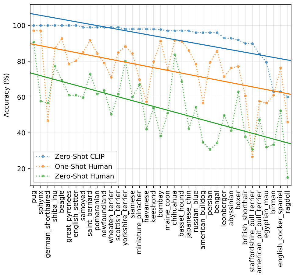
Five people each looked at 3669 images from the Oxford-IIIT Pets test split and chose which of 37 cat or dog breeds matched, or answered “I don’t know”. They were given zero, one, or two example images per breed.
| Accuracy | Majority Vote on Full Dataset | Accuracy on Guesses | Majority Vote Accuracy on Guesses | |
|---|---|---|---|---|
| Zero-shot human | 53.7 | 57.0 | 69.7 | 63.9 |
| Zero-shot CLIP | 93.5 | 93.5 | 93.5 | 93.5 |
| One-shot human | 75.7 | 80.3 | 78.5 | 81.2 |
| Two-shot human | 75.7 | 85.0 | 79.2 | 86.1 |
Humans went from 54% to 76% with a single example per class, and the marginal gain from a second example is minimal. Crucially, the gain from zero to one shot is almost entirely on images the participants were uncertain about. Humans know what they do not know, and spend the example filling exactly that gap.
CLIP does not. Its few-shot evaluations make no effective use of prior knowledge, which produces the counter-intuitive drop in performance when moving from zero-shot to one-shot fitting a linear classifier on its features.
Where CLIP fails
- Fine-grained classification. Differentiating models of cars, species of flowers and variants of aircraft.
- Abstract and systematic tasks. Counting the number of objects in an image.
- Genuinely novel tasks. Classifying the distance to the nearest car is near random. The authors are confident many such tasks remain.
- Truly out-of-distribution data. CLIP learns a high quality semantic OCR representation for digitally rendered text, yet achieves only 88% accuracy on the handwritten digits of MNIST — worse than logistic regression on raw pixels. Retrieval confirms almost no MNIST-like images exist in the pre-training data. CLIP does not solve brittle generalisation; it hopes that a large enough dataset makes everything in-distribution, an assumption MNIST violates.
Structural limits
- Zero-shot classification is limited to choosing among the concepts in a given classifier. It cannot generate novel output the way image captioning could — and the caption baseline was far less compute-efficient.
- Data efficiency is not addressed, only compensated for. At one image per second, iterating the 12.8 billion images seen over 32 epochs would take 405 years.
- Scaling is an expensive route out: roughly a 1000x increase in compute is estimated for zero-shot CLIP to reach overall state of the art, which is infeasible on current hardware.
- The methodology has its own limits. Full validation sets were repeatedly queried to guide development, which is unrealistic for a true zero-shot scenario, and the 27-dataset suite is co-adapted with CLIP’s development.
Section 8 of the paper places CLIP among joint vision-language models such as ViLBERT and UNITER. Those combine three or more pre-trained subsystems with dense joint attention. CLIP’s only cross-modal interaction is a single dot product.
Learning outcomes
- limitations-and-human-baseline Identify where CLIP fails, and compare its sample efficiency with a human’s.
Bias and broader impacts
CLIP makes it possible to create your own classes without re-training — to “roll your own classifier”. That capability magnifies existing issues. One can give it images of cats and dogs and ask it to classify cats, or give it images from a department store and ask it to classify shoplifters, a task with significant social implications and for which AI may be unfit.
Bias comes with the data
Algorithmic decisions, training data, and class design — the choice of how classes are defined and taxonomised — all contribute to social bias. Class design is particularly relevant here, since any developer can define a class and the model will return some result.
Zero-shot CLIP was asked to classify 10,000 images from the FairFace dataset. Alongside the FairFace classes, seven further labels were added: animal, gorilla, chimpanzee, orangutan, thief, criminal and suspicious person.
- 4.9% of images were misclassified into one of the non-human classes. Images labelled ‘Black’ had the highest rate, approximately 14%, while all other races were under 8%. People aged 0–20 also reached 14%.
- 16.5% of male images were misclassified into crime-related classes, against 9.8% of female images. People aged 0–20 were most affected at roughly 18%, against about 12% for ages 20–60 and 0% for over 70.
Class design changes the harm
Adding a single class changes the result. With child added to the same label set, the proportion of people under 20 classified into crime-related or non-human categories fell sharply — for ages 0–2, from 30.3% to 2.3%; for ages 3–9, from 35.0% to 4.3%.
That is a consequential finding. The deployer, not only the trainer, determines how harm is distributed.
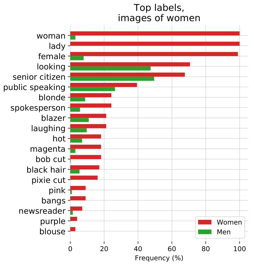
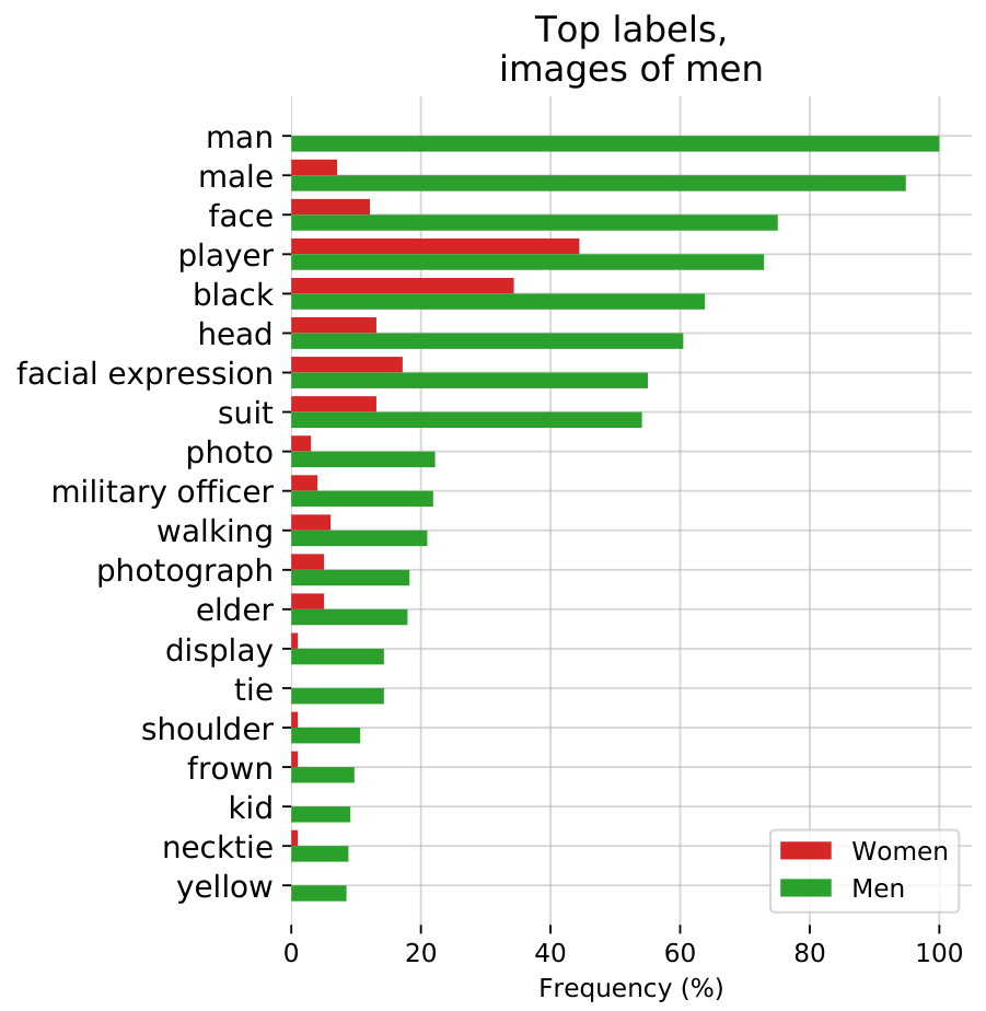
A parallel experiment on images of Members of Congress makes the same point about thresholds. At a 4% probability threshold the highest-probability labels across both genders are “lawmaker”, “legislator” and “congressman”. Lower the threshold to 0.5% and labels such as nanny and housekeeper begin appearing for women, while prisoner and mobster appear for men. Given the combined label set returned by Google Cloud Vision, Amazon Rekognition and Microsoft Azure Computer Vision, CLIP attached hair and appearance labels — brown hair, blonde, blond — disproportionately to women, and high-status occupations such as executive and doctor disproportionately to men. Of the only four occupations attached more often to women, three were newscaster, television presenter and newsreader.
A linear probe on CLIP features beats the FairFace model and the Instagram model on race, gender and age classification. That does not make it fair. Higher accuracy on underrepresented groups might be used by a company to justify deploying facial recognition, and then to deploy it in ways that affect demographic groups disproportionately.
Surveillance
The authors include surveillance deliberately, not enthusiastically, because its societal implications make it worth predicting.
- CCTV scene classification. On 515 surveillance images from 12 video sequences, coarse classification — identifying the main subject, with at least 6 options — reached 91.8% top-1. Under a stress test that added a “close” caption, such as parking lot with white car against parking lot with red car, accuracy fell to 51.1%, with the model choosing the close answer 40.7% of the time. Fine-grained detection of the presence or absence of small objects was near random.
- Identity recognition. On ‘in the wild’ CelebA images, zero-shot top-1 accuracy was 59.2% over 100 classes and 43.3% over 1,000.
Neither result is competitive with production systems such as Google’s Celebrity Recognition, and CLIP is not designed for detection or segmentation. What is noteworthy is that these numbers required no task-specific dataset at all. CLIP could enable bespoke, niche surveillance uses for which no well-tailored model exists, and lower the skill required to build them.
Future work
The paper closes this section by asking the community to characterise models before deploying them: identify beneficial downstream uses early, surface tasks whose sensitivity may call for policymaker intervention, characterise biases so others know where to intervene, and build suites of tests that evaluate systems like CLIP earlier in the development cycle.
Learning outcomes
- bias-and-impacts Assess the biases CLIP inherits from uncurated web data and the deployment risks that follow.
Concepts
- prompt-engineering-and-ensembling shows that prompt and class design choices strongly influence model output biases
- zero-shot-transfer probes zero-shot classification for societal and representational harms on face datasets
Conclusion
The paper’s own summary is short. It asked whether the success of task-agnostic web-scale pre-training in NLP transfers to another domain, and found that adopting the same formula produces similar behaviours in computer vision. To optimise their training objective, CLIP models learn to perform a wide variety of tasks during pre-training. That task learning is then reached through natural language prompting, which enables zero-shot transfer to many existing datasets. At sufficient scale the approach can be competitive with task-specific supervised models, although there is still room for much improvement.
Carry these away.
Natural language is a supervision signal that scales with the web rather than with an annotation budget.
No annotator has to be hired, and the label space is never closed. That is what allowed 400 million pairs where prior work had a hundred thousand.
Choosing the easier proxy task is what made the training compute affordable.
Predicting which caption goes with an image rather than which words it contains bought 4x over a bag-of-words baseline, which was itself 3x faster than generative captioning.
The text encoder is a hypernetwork, so any list of class names is a classifier.
76.2% top-1 on ImageNet with none of its 1.28 million labelled images, and a win over a supervised ResNet-50 linear probe on 16 of 27 datasets.
How you write the prompt is part of the model.
Prompt engineering and ensembling are worth almost 5% on ImageNet, and are free once the averaged text embeddings are cached.
Not fitting a dataset is what buys robustness to shifts of it.
Zero-shot CLIP closes up to 75% of the robustness gap. Adapting it with a linear probe raises ImageNet accuracy by 9.2% and gives that robustness back.
The failures are as informative as the successes.
Counting, fine-grained species and models, distance estimation, and 88% on MNIST. A human given one example gains 22 points; CLIP given one example gets worse.
Uncurated data and open class design put the consequences in the deployer’s hands.
4.9% of FairFace images fell into non-human classes, and adding a single
childlabel changed the distribution of that harm dramatically.
Where this goes next is CLIP Guided Image Diffusion. We now hold both halves of the mechanism. A diffusion model can be steered by the gradient of any differentiable score, and CLIP supplies a score between a text prompt and an image, computed as a single dot product in a shared space. The next unit works through classifier-guided diffusion in detail — the architecture ablations and the fidelity-diversity trade-off — and then GLIDE, which applies guidance to text-to-image generation and compares CLIP guidance against classifier-free guidance directly.
Keep this unit’s caution attached to that. A CLIP score is optimisable, and a generator that optimises it can find samples that score well and look wrong.
Learning outcomes
- natural-language-supervision Explain why raw text is a better supervision signal than a fixed set of labels.
- webimagetext-dataset Describe how the 400M-pair WebImageText dataset was constructed and why its scale matters.
- contrastive-objective Write the symmetric contrastive objective CLIP is trained on and explain its efficiency.
- architecture-and-scaling Describe CLIP’s dual-encoder architecture and how each side is scaled.
- zero-shot-classification Build a zero-shot classifier from class names, using prompt engineering and ensembling.
- representation-quality Evaluate CLIP’s features with linear probes and few-shot transfer, and read the results.
- effective-robustness Explain effective robustness and why zero-shot CLIP degrades less under distribution shift.
- limitations-and-human-baseline Identify where CLIP fails, and compare its sample efficiency with a human’s.
- bias-and-impacts Assess the biases CLIP inherits from uncurated web data and the deployment risks that follow.
References
- Radford, Alec, et al. “Learning transferable visual models from natural language supervision.” International conference on machine learning. PmLR, 2021.