Lecture notes — 2022 Classifier Free Diffusion Guidance
ver. 1.0.0, 2022_classifier_free_diffusion_guidance
← 2022 Classifier Free Diffusion Guidance
ver. 1.0.0 · 2026-08-22 10:23:24
Where we are: removing the second model
In CLIP Guided Image Diffusion you met two ways to steer a diffusion model, and both of them needed a second trained network. Classifier guidance shifted the reverse-process mean by the gradient of a classifier trained on noised inputs. CLIP guidance swapped that classifier for an image-text dot product, which bought arbitrary text prompts at the same structural price. GLIDE’s human evaluation preferred classifier-free guidance over CLIP guidance, but the method itself was used there without derivation.
Two objections survived that unit.
Guidance required a second network trained on noised inputs. A pre-trained classifier does not work, because it has never seen \(\mathbf{z}_\lambda\).
That complicates the training pipeline: two models, two training runs, and a noise schedule that both must agree on.
Optimising a classifier’s score looks uncomfortably like an adversarial attack on the very metric being reported.
Inception Score and FID are both computed with a classifier. Ascending a classifier gradient to raise them is at least suspicious.
Ho and Salimans remove the classifier entirely. This unit derives their method in full. It is the paper that gave the field the guidance scale that every text-to-image system now exposes as a slider, and the whole of it fits in two lines of code: drop the conditioning during a small fraction of training, and at sampling time run the model twice and extrapolate.
We motivate the outcomes here and derive the method in the sections that follow.
Ho, Jonathan, and Tim Salimans. “Classifier-free diffusion guidance.” arXiv preprint arXiv:2207.12598 (2022). A short version appeared at the NeurIPS 2021 Workshop on Deep Generative Models and Downstream Applications.
Learning outcomes
- classifier-guidance-as-score Recast classifier guidance as an additive term on the score, and state its costs.
- joint-training Train one diffusion model to be conditional and unconditional at once.
- cfg-sampling-rule Apply the classifier-free guidance extrapolation at sampling time.
What you will be able to do
score-view— Express diffusion sampling in terms of score estimates rather than noise predictions.classifier-guidance-as-score— Recast classifier guidance as an additive term on the score, and state its costs.joint-training— Train one diffusion model to be conditional and unconditional at once.cfg-sampling-rule— Apply the classifier-free guidance extrapolation at sampling time.guidance-strength-sweep— Sweep the guidance strength \(w\) and read the resulting fidelity-diversity curve.tuning-p-uncond-and-steps— Choose the unconditional training probability and the number of sampling steps.non-adversarial-and-limits— Argue that the quality gains are generative rather than adversarial, and state the method’s costs.
What we will cover
- Classifier-free guidance — a guidance method that adjusts the score direction by linearly combining conditional and unconditional score estimates drawn from a single model.
- Joint conditional/unconditional training — a training technique in which the conditioning label is randomly dropped with probability \(p_\text{uncond}\), so that one network learns both distributions.
- Guidance strength FID/IS trade-off — the operational trade-off by which increasing guidance strength improves Inception Score at the cost of FID and of sample diversity.
- Implicit classifier interpretation — the framing under which classifier-free guidance steps in the direction of an implicit Bayes classifier derived from generative scores.
The score view of diffusion
The paper works in continuous time. There is no index \(t\) running over \(T\) steps. Instead the forward process is indexed by \(\lambda\), and the whole latent trajectory is \(\mathbf{z} = \{\mathbf{z}_\lambda \mid \lambda \in [\lambda_{\min}, \lambda_{\max}]\}\). The forward process is the variance-preserving Markov process
\[q(\mathbf{z}_\lambda|\mathbf{x}) = \mathcal{N}(\alpha_\lambda \mathbf{x}, \sigma_\lambda^2 \mathbf{I}), \quad \alpha_\lambda^2 = 1/(1+e^{-\lambda}), \quad \sigma_\lambda^2 = 1 - \alpha_\lambda^2 .\]
Since \(\lambda = \log \alpha_\lambda^2/\sigma_\lambda^2\), the index \(\lambda\) is the log signal-to-noise ratio of \(\mathbf{z}_\lambda\). The forward process runs in the direction of decreasing \(\lambda\). Sampling runs the other way, along an increasing sequence \(\lambda_{\min} = \lambda_1 < \cdots < \lambda_T = \lambda_{\max}\).
The reverse process and its parameterization
The reverse process starts from \(p_\theta(\mathbf{z}_{\lambda_{\min}}) = \mathcal{N}(\mathbf{0}, \mathbf{I})\) and applies transitions whose mean \(\tilde{\boldsymbol\mu}_{\lambda'|\lambda}(\mathbf{z}_\lambda, \mathbf{x}_\theta(\mathbf{z}_\lambda))\) comes from plugging an estimate \(\mathbf{x}_\theta(\mathbf{z}_\lambda) \approx \mathbf{x}\) into the true reverse transition \(q(\mathbf{z}_{\lambda'}|\mathbf{z}_\lambda, \mathbf{x})\). The estimate is written in terms of \(\epsilon\)-prediction,
\[\mathbf{x}_\theta(\mathbf{z}_\lambda) = (\mathbf{z}_\lambda - \sigma_\lambda \epsilon_\theta(\mathbf{z}_\lambda))/\alpha_\lambda ,\]
and the network is trained on the plain denoising objective \(\mathbb{E}_{\epsilon,\lambda}[\|\epsilon_\theta(\mathbf{z}_\lambda) - \epsilon\|_2^2]\), with \(\epsilon \sim \mathcal{N}(\mathbf{0},\mathbf{I})\), \(\mathbf{z}_\lambda = \alpha_\lambda \mathbf{x} + \sigma_\lambda \epsilon\), and \(\lambda\) drawn from a distribution \(p(\lambda)\) over \([\lambda_{\min}, \lambda_{\max}]\). When \(p(\lambda)\) is uniform this objective is proportional to the variational lower bound; the authors instead sample \(\lambda = -2\log\tan(au+b)\) for uniform \(u \in [0,1]\), a bounded hyperbolic secant distribution inspired by the cosine noise schedule.
Noise prediction is score estimation
Here is the sentence the whole unit rests on. Because the loss is denoising score matching at every \(\lambda\),
\[\epsilon_\theta(\mathbf{z}_\lambda) \approx -\sigma_\lambda \nabla_{\mathbf{z}_\lambda} \log p(\mathbf{z}_\lambda) .\]
The network output is a scaled estimate of the score of the noisy data distribution. That is what licenses adding things to \(\epsilon_\theta\) and calling the result a different distribution — an addition to \(\epsilon_\theta\) is a multiplicative reweighting of \(p\). Conditional modelling changes nothing structural: the function approximator simply receives \(\mathbf{c}\) as an extra input, giving \(\epsilon_\theta(\mathbf{z}_\lambda, \mathbf{c})\).
The paper is careful about a caveat we will need in the last section: because \(\epsilon_\theta\) is defined by an unconstrained neural network, there need not exist any scalar potential whose gradient is \(\epsilon_\theta\). The approximation above holds in the sense of the training objective, not as an identity of vector fields.
The sampler variance is a log-space interpolation, \((\hat\sigma_{\lambda'|\lambda}^2)^{1-v}(\sigma_{\lambda|\lambda'}^2)^{v}\), with \(v\) a constant hyperparameter rather than a learned function of \(\mathbf{z}_\lambda\). The variances coincide as \(\lambda' \to \lambda\), so \(v\) matters only at the non-infinitesimal step sizes used in practice.
GANs and flow-based models can trade diversity for individual fidelity by shrinking the range of their noise inputs — truncation in BigGAN, low-temperature sampling in Glow. Diffusion models have no such dial. Scaling the model scores, or decreasing the variance of the Gaussian noise in the reverse process, produces blurry low-quality samples.
Learning outcomes
- score-view Express diffusion sampling in terms of score estimates rather than noise predictions.
Classifier guidance in score form
Dhariwal and Nichol obtained a truncation-like effect by modifying the diffusion score with the gradient of an auxiliary classifier \(p_\theta(\mathbf{c}|\mathbf{z}_\lambda)\):
\[\tilde\epsilon_\theta(\mathbf{z}_\lambda, \mathbf{c}) = \epsilon_\theta(\mathbf{z}_\lambda, \mathbf{c}) - w\sigma_\lambda \nabla_{\mathbf{z}_\lambda} \log p_\theta(\mathbf{c}|\mathbf{z}_\lambda) \approx -\sigma_\lambda \nabla_{\mathbf{z}_\lambda}\!\left[\log p(\mathbf{z}_\lambda|\mathbf{c}) + w \log p_\theta(\mathbf{c}|\mathbf{z}_\lambda)\right],\]
where \(w\) controls the strength. Read the right-hand side through the score view of the previous section: it is \(-\sigma_\lambda\) times the gradient of a log-density, so using \(\tilde\epsilon_\theta\) in place of \(\epsilon_\theta\) during sampling yields approximate samples from
\[\tilde p_\theta(\mathbf{z}_\lambda|\mathbf{c}) \propto p_\theta(\mathbf{z}_\lambda|\mathbf{c})\, p_\theta(\mathbf{c}|\mathbf{z}_\lambda)^w .\]
Raising the classifier term to the power \(w\) up-weights data the classifier assigns confidently to the correct label. That is exactly what Inception Score rewards, by design — so setting \(w > 0\) improves IS at the expense of sample diversity.
The toy case first
The paper’s 2D example makes the geometry visible. Take three classes whose class-conditional distributions are isotropic Gaussians. Solve the guided density \(\tilde p_\theta \propto p_\theta(\mathbf{z}_\lambda|\mathbf{c})p_\theta(\mathbf{c}|\mathbf{z}_\lambda)^w\) numerically and plot it.
Each guided conditional is markedly non-Gaussian, even though every unguided conditional was Gaussian.
Guidance is not a rescaling of the conditional. It reshapes it.
As \(w\) grows, each conditional places mass farther from the other classes, toward the directions of high confidence given by logistic regression.
Mass concentrates into smaller regions. That is the toy version of the IS boost and the diversity loss seen on ImageNet.

What it costs, and the crack in it
The method needs a classifier \(p_\theta(\mathbf{c}|\mathbf{z}_\lambda)\) trained on noisy \(\mathbf{z}_\lambda\) — a standard pre-trained classifier cannot be substituted — and a backward pass through it at every sampling step.
There is also a redundancy worth noticing. Applying classifier guidance with weight \(w+1\) to an unconditional model gives the same target as weight \(w\) on a conditional model, since \(p_\theta(\mathbf{z}_\lambda|\mathbf{c})p_\theta(\mathbf{c}|\mathbf{z}_\lambda)^w \propto p_\theta(\mathbf{z}_\lambda)p_\theta(\mathbf{c}|\mathbf{z}_\lambda)^{w+1}\). The conditional score and the unconditional score differ by exactly one classifier gradient. Ho and Salimans stay with the conditional setup — Dhariwal and Nichol got their best results there — but the identity is the hinge on which the next section turns.
Learning outcomes
- classifier-guidance-as-score Recast classifier guidance as an additive term on the score, and state its costs.
Concepts
- guidance-strength-tradeoff introduces the trade-off mechanism between perceptual quality metrics (IS) and diversity (FID) via classifier guidance
Classifier-free guidance
Rather than train a separate classifier, train an unconditional diffusion model \(p_\theta(\mathbf{z})\) alongside the conditional \(p_\theta(\mathbf{z}|\mathbf{c})\). Both are parameterized by a single neural network: the unconditional score is obtained by feeding a null token \(\varnothing\) in place of the class identifier,
\[\epsilon_\theta(\mathbf{z}_\lambda) = \epsilon_\theta(\mathbf{z}_\lambda, \mathbf{c} = \varnothing).\]
Joint training
Joint conditional/unconditional training means randomly setting \(\mathbf{c}\) to \(\varnothing\) with probability \(p_\text{uncond}\), a hyperparameter. Nothing else changes.
Algorithm 1 Joint training a diffusion model with classifier-free guidance
Require: p_uncond: probability of unconditional training
1: repeat
2:   (x, c) ~ p(x, c)                 # Sample data with conditioning from the dataset
3:   c <- null  with probability p_uncond   # Randomly discard conditioning
4:   lambda ~ p(lambda)               # Sample log SNR value
5:   eps ~ N(0, I)
6:   z_lambda = alpha_lambda * x + sigma_lambda * eps
7:   Take gradient step on grad_theta || eps_theta(z_lambda, c) - eps ||^2
8: until converged
Training two separate models would also work. The authors choose joint training because it is extremely simple to implement, does not complicate the training pipeline, and does not increase the total number of parameters.
The sampling rule
Sampling uses a linear combination of the two score estimates — equation (6) of the paper:
\[\tilde\epsilon_\theta(\mathbf{z}_\lambda, \mathbf{c}) = (1+w)\,\epsilon_\theta(\mathbf{z}_\lambda, \mathbf{c}) - w\,\epsilon_\theta(\mathbf{z}_\lambda).\]
Write it as \(\epsilon_\theta(\mathbf{z}_\lambda,\mathbf{c}) + w[\epsilon_\theta(\mathbf{z}_\lambda,\mathbf{c}) - \epsilon_\theta(\mathbf{z}_\lambda)]\) and the geometry is plain: start at the conditional prediction and keep going, directly away from the unconditional one. The difference vector is what the condition contributes; \(w\) says how far past it to travel. At \(w = 0\) the rule collapses to ordinary conditional sampling.
Algorithm 2 Conditional sampling with classifier-free guidance
Require: w: guidance strength; c: conditioning information
Require: lambda_1, ..., lambda_T: increasing log SNR sequence
1: z_1 ~ N(0, I)
2: for t = 1, ..., T do
3:   eps~_t = (1+w) eps_theta(z_t, c) - w eps_theta(z_t)
     # Sampling step (could be replaced by another sampler, e.g. DDIM)
4:   x~_t = (z_t - sigma_{lambda_t} eps~_t) / alpha_{lambda_t}
5:   z_{t+1} ~ N(mu~(z_t, x~_t), (sigma~^2)^{1-v}(sigma^2)^v)  if t < T else z_{t+1} = x~_t
6: end for
7: return z_{T+1}
The implicit classifier
Why should this reproduce classifier guidance? Consider the implicit classifier defined by Bayes’ rule from the generative model, \(p^i(\mathbf{c}|\mathbf{z}_\lambda) \propto p(\mathbf{z}_\lambda|\mathbf{c})/p(\mathbf{z}_\lambda)\). Given exact scores \(\epsilon^*(\mathbf{z}_\lambda, \mathbf{c})\) and \(\epsilon^*(\mathbf{z}_\lambda)\), its gradient is a difference of two scores:
\[\nabla_{\mathbf{z}_\lambda} \log p^i(\mathbf{c}|\mathbf{z}_\lambda) = -\frac{1}{\sigma_\lambda}\left[\epsilon^*(\mathbf{z}_\lambda,\mathbf{c}) - \epsilon^*(\mathbf{z}_\lambda)\right].\]
Substitute that into the classifier-guidance formula of the previous section and the \(\sigma_\lambda\) cancels, leaving \(\tilde\epsilon^*(\mathbf{z}_\lambda,\mathbf{c}) = (1+w)\epsilon^*(\mathbf{z}_\lambda,\mathbf{c}) - w\epsilon^*(\mathbf{z}_\lambda)\) — the shape of equation (6), with no classifier anywhere in it.
The paper insists that \(\tilde\epsilon^*\) differs fundamentally from \(\tilde\epsilon_\theta\). The former is built from a genuine scaled classifier gradient; the latter from the estimate \(\epsilon_\theta(\mathbf{z}_\lambda,\mathbf{c}) - \epsilon_\theta(\mathbf{z}_\lambda)\), which is not in general the gradient of any classifier, because both terms are outputs of unconstrained networks. Equation (6) is inspired by the implicit classifier; it does not implement one.
Nor is it obvious that inverting a generative model by Bayes’ rule gives a useful classifier at all. Grandvalet and Bengio found discriminative models generally beat implicit classifiers derived from generative ones, even when the generative specification exactly matches the data. Under misspecification — which is our case — Bayes-derived classifiers can be inconsistent, and all guarantees are lost. The justification is therefore empirical, which is what the next section supplies.
Learning outcomes
- joint-training Train one diffusion model to be conditional and unconditional at once.
- cfg-sampling-rule Apply the classifier-free guidance extrapolation at sampling time.
Concepts
- classifier-free-guidance presents the formal definition, algorithms, and score formula for classifier-free guidance
- joint-conditional-unconditional-training details the joint training strategy using label dropout to model conditional and unconditional distributions with one network
- implicit-classifier derives classifier-free guidance as an approximation of an implicit Bayes classifier gradient
Sweeping the guidance strength
The experiments run on area-downsampled class-conditional ImageNet, the standard setting for studying FID/IS trade-offs since BigGAN. The architectures and hyperparameters are those of Dhariwal and Nichol, apart from the continuous-time training above — settings tuned for classifier guidance, and so possibly suboptimal here. Note also that amortizing the conditional and unconditional models into one architecture, with no extra classifier, uses less model capacity than the prior work being compared against. Log SNR endpoints were \(\lambda_{\min} = -20\) and \(\lambda_{\max} = 20\); the \(64\times64\) models used \(v = 0.3\) and 400 thousand training steps, the \(128\times128\) models \(v = 0.2\) and 2.7 million.
The sweep covers \(w \in \{0, 0.1, 0.2, \ldots, 4\}\), with FID and Inception Score computed from 50000 samples at each value.
Reading the curve
At \(64\times64\) with \(p_\text{uncond} = 0.1\), the numbers move like this:
| \(w\) | FID | IS |
|---|---|---|
| 0.0 | 1.80 | 53.71 |
| 0.1 | 1.55 | 66.11 |
| 0.3 | 3.03 | 92.8 |
| 1.0 | 12.6 | 170.1 |
| 4.0 | 26.22 | 260.2 |
Inception Score climbs the whole way. FID improves once, at \(w = 0.1\), then deteriorates steadily. The best FID comes from a small amount of guidance (\(w = 0.1\) or \(w = 0.3\), depending on the dataset) and the best IS from strong guidance (\(w \ge 4\)); between the extremes there is a clear trade-off.
Section 4.1 of the paper describes this as “FID monotonically decreasing and IS monotonically increasing with \(w\)”. Tables 1 and 2 show FID increasing — worsening — above the optimum, and the accompanying figures show the same. Trust the tables. FID has a minimum at small nonzero \(w\).
At \(128\times128\) the picture is the same with a shifted optimum: FID 7.27 unguided, a minimum of 2.43 at \(w = 0.3\), and 21.53 at \(w = 4.0\) where IS reaches 421.03. Two comparisons follow. At \(w = 0.3\) the FID of 2.43 beats the classifier-guided ADM-G at 2.97. At \(w = 4.0\) the model beats BigGAN-deep on both FID and IS when BigGAN-deep is evaluated at its best-IS truncation level (FID 25, IS 253). A purely generative model reproduces the truncation effect.
What it looks like
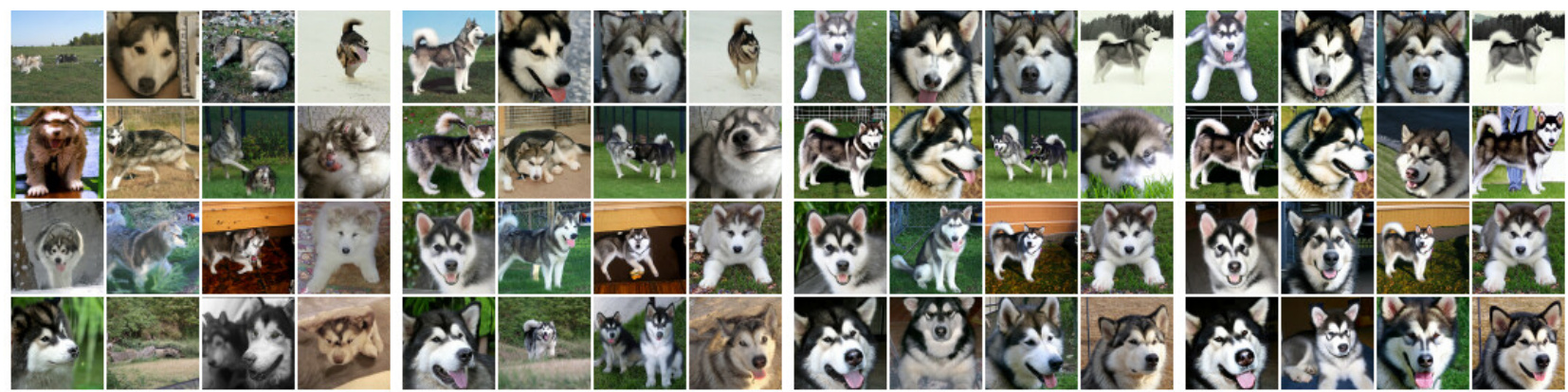
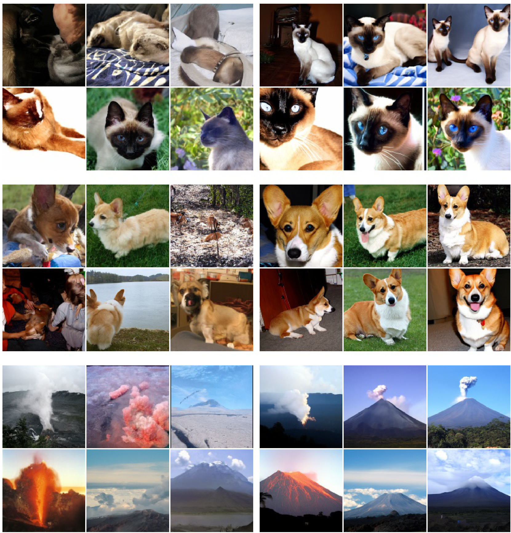
The sample grids in Appendix A use the same random seed within each subfigure, so the change is attributable to \(w\) alone.
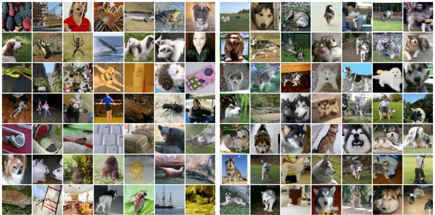
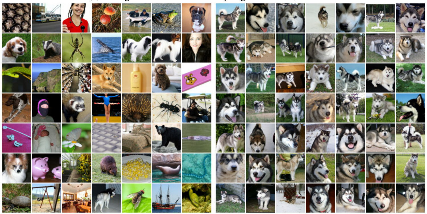
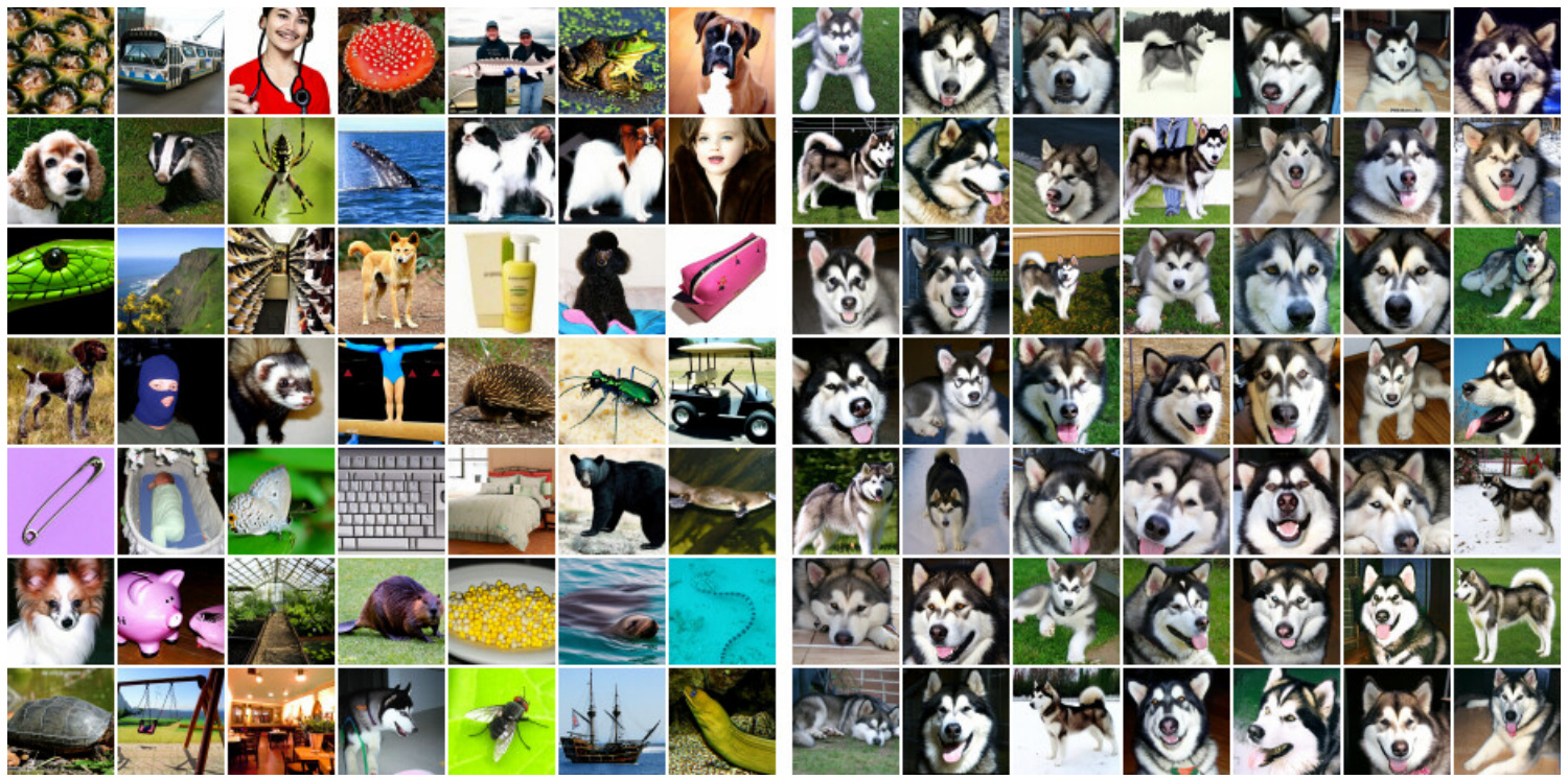
Increasing guidance strength decreases sample variety and increases individual sample fidelity. The \(128\times128\) grids repeat the pattern from FID 7.27 / IS 82.45 unguided to FID 21.53 / IS 421.03 at \(w = 4.0\).
Learning outcomes
- guidance-strength-sweep Sweep the guidance strength \(w\) and read the resulting fidelity-diversity curve.
Concepts
- classifier-free-guidance evaluates classifier-free guidance across a range of guidance values \(w\) on ImageNet
- guidance-strength-tradeoff quantifies the FID versus Inception Score Pareto curves as guidance strength \(w\) increases
Tuning \(p_\text{uncond}\) and the sampling steps
Two knobs remain. Both were measured.
How often to drop the label
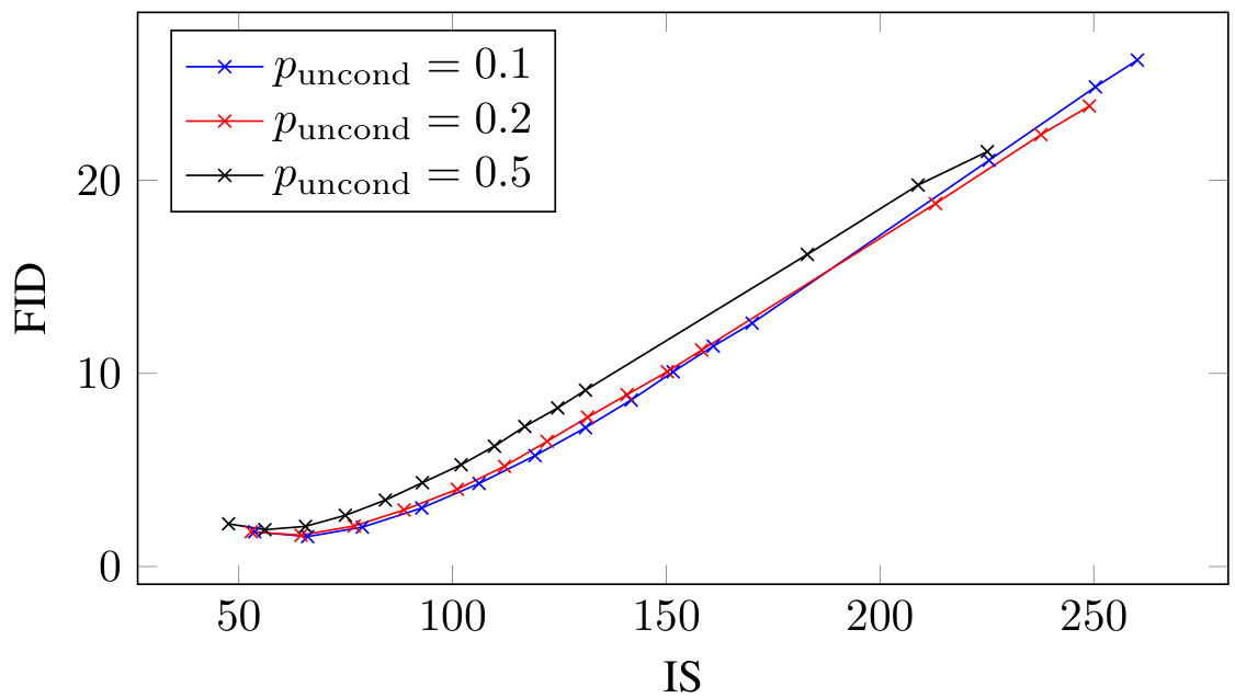
\(p_\text{uncond}\) is the only hyperparameter classifier-free guidance introduces at training time. The authors trained \(64\times64\) models at \(p_\text{uncond} \in \{0.1, 0.2, 0.5\}\), all for 400 thousand steps, and evaluated across guidance strengths.
\(p_\text{uncond} = 0.5\) performs consistently worse than \(0.1\) or \(0.2\) across the entire IS/FID frontier.
At \(w = 0.1\) the FIDs are 1.55, 1.62 and 1.91 for \(0.1\), \(0.2\) and \(0.5\); the corresponding Inception Scores are 66.11, 64.58 and 56.1. The gap does not close anywhere along the sweep.
\(p_\text{uncond} \in \{0.1, 0.2\}\) perform about equally well as each other.
There is no fine tuning to be done here. Pick either.
The conclusion the paper draws is the interesting part: only a relatively small portion of model capacity needs to be dedicated to the unconditional task in order to produce guided scores effective for sample quality. Dhariwal and Nichol reported the mirror-image finding for classifier guidance, where relatively small, low-capacity classifiers sufficed.
How many sampling steps
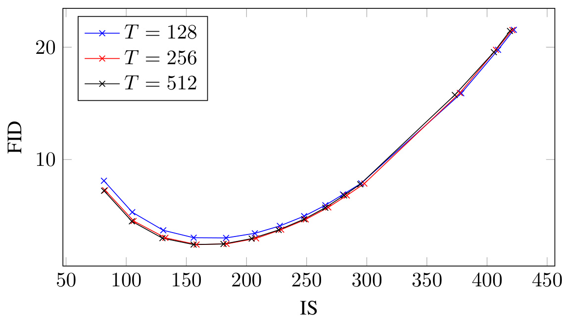
On the \(128\times128\) model the authors varied \(T \in \{128, 256, 1024\}\) over a range of guidance strengths. Sample quality improves as \(T\) increases, as expected, and \(T = 256\) attains a good balance between quality and sampling speed. The gain from 256 to 1024 is slight — at \(w = 0.3\), FID 2.43 either way.
\(T = 256\) is approximately the step count used by ADM-G, which this model outperforms. But every step here evaluates the denoising model twice, once for \(\epsilon_\theta(\mathbf{z}_\lambda,\mathbf{c})\) and once for \(\epsilon_\theta(\mathbf{z}_\lambda)\). Since the architecture is the same as ADM-G’s, the fair comparison on sampling speed is the \(T = 128\) setting — and that setting underperforms ADM-G on FID (3.04 against 2.97 at \(w = 0.3\)).
Key ideas
- \(p_\text{uncond} \approx 0.1\)–\(0.2\); \(0.5\) is measurably worse and there is nothing between \(0.1\) and \(0.2\) to choose.
- \(T = 256\) balances quality against speed on \(128\times128\); \(T = 1024\) buys almost nothing.
- Report guidance costs in network evaluations, which are \(2T\), not in steps.
Learning outcomes
- tuning-p-uncond-and-steps Choose the unconditional training probability and the number of sampling steps.
Concepts
- joint-conditional-unconditional-training studies the effect of varying \(p_\text{uncond}\) during joint training
- guidance-strength-tradeoff analyzes how different unconditional training probabilities affect the achievable FID/IS frontier
- classifier-free-guidance evaluates sampling step requirements when generating with classifier-free guidance
Is guidance adversarial?
We can now settle the objection raised in the opening. The worry was that classifier guidance raises Inception Score by sharpening a classifier’s output, and that IS is itself computed with a classifier — so the reported gain might be metric gaming rather than better images.
Classifier-free guidance escapes the charge on two grounds, and the paper states both.
There is no classifier gradient in equation (6). Taking a step in the \(\tilde\epsilon_\theta\) direction cannot be interpreted as a gradient-based adversarial attack on an image classifier, because no classifier is evaluated.
The result is that boosting the classifier-based IS and FID metrics is accomplished by a pure generative model whose sampling procedure never touches a classifier gradient.
The score estimates are non-conservative vector fields. They come from unconstrained neural networks, so in general no scalar potential — no classifier log likelihood — exists for which \(\tilde\epsilon_\theta\) is the classifier-guided score.
Classifier gradients are conservative by construction. The guided direction here does not resemble one at all, so there is nothing to ascend adversarially.
What it does cost
The paper is equally direct about the price.
- Diversity, genuinely. Guidance increases fidelity at the expense of diversity. This is not a metric artefact; the FID curve of the sweep section reports it faithfully. The authors raise it as a deployment concern: sample diversity matters where parts of the data are underrepresented, and boosting quality while preserving diversity is left as future work.
- Sampling speed. Classifiers can be smaller and faster than generative models, so classifier-guided sampling may well be faster than running two forward passes of the diffusion model. Injecting the conditioning late in the network might mitigate this; the paper leaves that unexplored.
- An unconditional model to train. In some cases even this is avoidable: when the class distribution is known and the classes are few, \(\sum_\mathbf{c} p(\mathbf{x}|\mathbf{c})p(\mathbf{c}) = p(\mathbf{x})\) recovers the unconditional score from conditional ones — at the cost of one forward pass per class, which is hopeless for high-dimensional conditioning.
The paper offers a one-sentence account of how guidance works: it decreases the unconditional likelihood of the sample while increasing the conditional likelihood. Classifier-free guidance achieves the decrease with a negative score term — the \(-w\,\epsilon_\theta(\mathbf{z}_\lambda)\) — which the authors note had not been explored before and may find other uses.
Learning outcomes
- non-adversarial-and-limits Argue that the quality gains are generative rather than adversarial, and state the method’s costs.
Closing the Generative Models module
Classifier-free guidance increases sample quality while decreasing sample diversity in diffusion models. It is classifier guidance without a classifier, and its results confirm that pure generative diffusion models can maximize classifier-based sample quality metrics while entirely avoiding classifier gradients.
Noise prediction is a scaled score estimate: \(\epsilon_\theta(\mathbf{z}_\lambda) \approx -\sigma_\lambda \nabla_{\mathbf{z}_\lambda}\log p(\mathbf{z}_\lambda)\).
That is what turns an arithmetic operation on network outputs into a statement about a distribution.
Classifier guidance samples from \(p_\theta(\mathbf{z}_\lambda|\mathbf{c})p_\theta(\mathbf{c}|\mathbf{z}_\lambda)^w\), and the classifier gradient it needs is a difference of two scores.
Both of those scores are things a diffusion model estimates directly, which is why the classifier turned out not to be fundamental.
One network learns both scores when the conditioning is replaced by \(\varnothing\) with probability \(p_\text{uncond}\).
No second model, no second training run, no extra parameters — a one-line change during training.
Sampling extrapolates: \(\tilde\epsilon_\theta = (1+w)\epsilon_\theta(\mathbf{z}_\lambda,\mathbf{c}) - w\epsilon_\theta(\mathbf{z}_\lambda)\).
\(w\) is a dial on a real trade-off, not a free improvement: best FID at small nonzero \(w\), best IS at large \(w\).
The gains are generative, not adversarial, because unconstrained score estimates are non-conservative.
The cost is paid instead in diversity and in doubled sampling compute.
The arc of the module
Look back across Generative Models as a whole. Chapter 17: Variational autoencoders gave latent variable models and the ELBO, with a learned encoder that could collapse. Chapter 18: Diffusion models replaced that encoder with a fixed noising chain, reducing the same bound to noise prediction. 2021 CLIP built a shared image-text space by contrastive learning at web scale. CLIP Guided Image Diffusion used gradients from a classifier or from CLIP to steer generation, and scaled it to text. This unit removed the external model and left a two-line rule that is now standard practice everywhere conditional diffusion is deployed.
One thread runs through all five: choose a tractable bound, make the stochastic part differentiable, and control the result with a single interpretable dial.
Learning outcomes
- score-view Express diffusion sampling in terms of score estimates rather than noise predictions.
- classifier-guidance-as-score Recast classifier guidance as an additive term on the score, and state its costs.
- joint-training Train one diffusion model to be conditional and unconditional at once.
- cfg-sampling-rule Apply the classifier-free guidance extrapolation at sampling time.
- guidance-strength-sweep Sweep the guidance strength \(w\) and read the resulting fidelity-diversity curve.
- tuning-p-uncond-and-steps Choose the unconditional training probability and the number of sampling steps.
- non-adversarial-and-limits Argue that the quality gains are generative rather than adversarial, and state the method’s costs.
References
- Ho, Jonathan, and Tim Salimans. “Classifier-free diffusion guidance.” arXiv preprint arXiv:2207.12598 (2022).