Lecture notes — Chapter 17: Variational autoencoders
ver. 1.0.0, chapter_17_variational_autoencoders
← Chapter 17: Variational autoencoders
ver. 1.0.0 · 2026-08-22 05:40:56
Where we are
This is the first unit of the Generative Models module, so there is no immediately preceding lesson to build on. What the unit does assume is the material of an introductory deep learning course: how a deep network computes a function, how backpropagation delivers gradients, and how stochastic gradient descent uses them.
Two further pieces of probability are used throughout. The first is marginalisation — recovering a distribution over one variable by integrating a joint distribution over the other. The second is the Kullback-Leibler divergence, a non-negative measure of the difference between two distributions, which is zero exactly when the two agree.
Everything before this point mapped an input to a prediction. Here the target is the data distribution itself.
What you will be able to do
latent-variable-models— Explain how a latent variable model describes a complex density by marginalising a joint distribution.nonlinear-latent-model— Describe the continuous nonlinear latent variable model defined by a decoder network and sample from it.derive-elbo— Explain why maximum likelihood is intractable here and derive the evidence lower bound with Jensen’s inequality.interpret-elbo— Interpret the ELBO as reconstruction minus KL, and explain exactly when the bound is tight.variational-approximation— Explain the encoder as an amortised variational approximation to the true posterior.vae-algorithm— Assemble encoder and decoder into a VAE and write down its training algorithm and loss.reparameterization-trick— Apply the reparameterization trick to backpropagate through a stochastic latent layer.vae-applications— Use a trained VAE to generate, to estimate sample probability, and to resynthesise data.disentanglement-and-limits— Modify the VAE loss for disentangled latents, and name the failure modes of the basic model.
What we will cover
The source for this unit is Understanding Deep Learning, Simon Prince, chapter 17. It introduces the following ideas.
- Latent variable models — probabilistic models that describe a complex observed density by marginalising over unobserved variables.
- Nonlinear latent variable model — a continuous latent variable passed through a deep network to set the parameters of the data distribution.
- Evidence lower bound (ELBO) — a tractable lower bound on the log evidence, used as the training objective.
- Variational approximation — replacing an intractable posterior by the closest member of a tractable family.
- Variational autoencoder (VAE) — the encoder-decoder architecture that computes and maximises the ELBO.
- Reparameterization trick — a rewriting of the sampling step that restores differentiability.
- Resynthesis and latent space manipulation — encoding real data, editing the code, and decoding again.
- Disentangled latent representations — latent axes that correspond one-to-one with independent real-world factors.
- Posterior collapse — the failure mode in which the encoder returns the prior for every input.
Opening: generative models and latents
Up to now our networks have been discriminative. Given an input \(x\), they predict an output \(y\). A generative model has a harder job. It must describe the whole data distribution \(Pr(x)\) well enough that we can draw new examples from it.
Prince opens the chapter by placing variational autoencoders alongside two other families. Generative adversarial networks learn a mechanism for creating samples that cannot be distinguished from the training examples \(\{x_i\}\). Variational autoencoders, like normalizing flows, are probabilistic generative models: they aim to learn a distribution \(Pr(x)\) over the data. After training it is possible to draw samples from that distribution. It is, however, not possible to evaluate the probability of a new example \(x^*\) exactly. That asymmetry — easy to sample, hard to score — is what the rest of the unit is about.
Prince is explicit on this point. It is common to talk about the VAE as if it is the model of \(Pr(x)\), but this is misleading. The VAE is a neural architecture designed to help learn the model for \(Pr(x)\). The final model contains neither the “variational” nor the “autoencoder” parts, and might be better described as a nonlinear latent variable model.
Images live in a very high dimensional space, so we cannot write \(Pr(x)\) down directly. The move we will build on is to introduce an unobserved latent variable \(z\) in a lower dimensional space, model the pair \((x, z)\), and recover \(Pr(x)\) by marginalising \(z\) away.
That move buys expressiveness and costs tractability. Simple expressions for the prior and the conditional can define a complicated marginal, but the marginal integral has no closed form, so maximum likelihood training is out of reach.
The rest of the unit is the repair, in four steps.
Define the evidence lower bound — a quantity we can compute that never exceeds the log-likelihood.
Jensen’s inequality is the tool that produces it.
Introduce an encoder network to supply the auxiliary distribution the bound needs.
Without it, the bound would have to be optimised separately for every training example.
Make the whole pipeline differentiable with the reparameterization trick.
A sampling step sits in the middle of the network, and gradients do not pass through it unaided.
Put a trained model to work: generation, probability estimation, resynthesis, and disentanglement.
We are motivating these here, not yet teaching them.
Learning outcomes
- latent-variable-models Explain how a latent variable model describes a complex density by marginalising a joint distribution.
- nonlinear-latent-model Describe the continuous nonlinear latent variable model defined by a decoder network and sample from it.
- derive-elbo Explain why maximum likelihood is intractable here and derive the evidence lower bound with Jensen’s inequality.
Latent variable models and mixtures
Latent variable models take an indirect approach to describing a probability distribution \(Pr(x)\) over a multi-dimensional variable \(x\). Instead of writing the expression for \(Pr(x)\) directly, we model a joint distribution \(Pr(x, z)\) of the data \(x\) and an unobserved hidden or latent variable \(z\). We then describe \(Pr(x)\) as a marginalisation of this joint probability:
\[Pr(x) = \int Pr(x, z)\, dz. \tag{17.1}\]
The joint probability is typically broken down using the rules of conditional probability, into the likelihood of the data with respect to the latent variable, \(Pr(x|z)\), and the prior \(Pr(z)\):
\[Pr(x) = \int Pr(x|z) Pr(z)\, dz. \tag{17.2}\]
This is a rather indirect approach, but it is useful because relatively simple expressions for \(Pr(x|z)\) and \(Pr(z)\) can define complex distributions \(Pr(x)\).
Example: mixture of Gaussians
The cleanest instance is the one where the latent variable is discrete, so the integral becomes a finite sum and everything can be computed exactly.
In a 1D mixture of Gaussians, the latent variable \(z\) is discrete and the prior \(Pr(z)\) is a categorical distribution with one probability \(\lambda_n\) for each possible value of \(z\). The likelihood \(Pr(x|z=n)\) of the data \(x\), given that the latent variable takes value \(n\), is normally distributed with mean \(\mu_n\) and variance \(\sigma_n^2\):
\[ \begin{aligned} Pr(z=n) &= \lambda_n \\ Pr(x|z=n) &= \text{Norm}_x\!\left[\mu_n, \sigma_n^2\right]. \end{aligned} \tag{17.3} \]
Here the latent variable is discrete, so we sum over its possible values to marginalise:
\[ \begin{aligned} Pr(x) &= \sum_{n=1}^{N} Pr(x, z=n) \\ &= \sum_{n=1}^{N} Pr(x|z=n) \cdot Pr(z=n) \\ &= \sum_{n=1}^{N} \lambda_n \cdot \text{Norm}_x\!\left[\mu_n, \sigma_n^2\right]. \end{aligned} \tag{17.4} \]
From simple expressions for the likelihood and prior, we describe a complex multi-modal probability distribution.
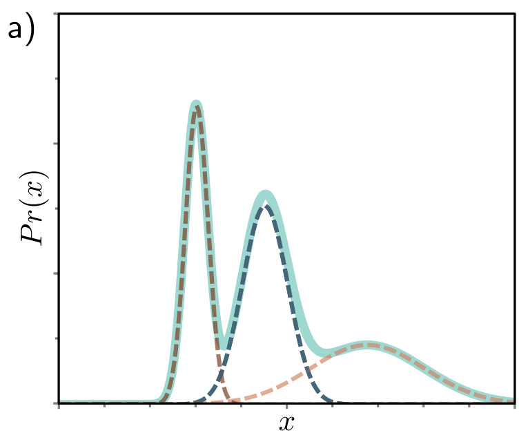
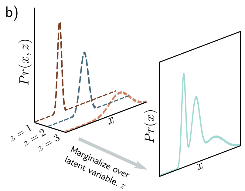
Read the latent variable here as an identity: \(z\) names which component generated the point. The prior \(\lambda_n\) says how often each component is chosen before we see anything, and the posterior \(Pr(z|x)\) says which component is responsible after we have seen \(x\).
Prince’s notation writes the parameters of a distribution inside square brackets, so \(\text{Norm}_x[\mu, \sigma^2]\) is a normal density over \(x\) with mean \(\mu\) and variance \(\sigma^2\). The subscript names the variable the density is over.
The takeaway carries forward unchanged: a simple prior plus a simple conditional can produce a complicated marginal. That is the whole trick, and it survives the move to a continuous \(z\).
Learning outcomes
- latent-variable-models Explain how a latent variable model describes a complex density by marginalising a joint distribution.
Concepts
- latent-variable-models introduces the definition of latent variable models via marginalisation over joint probability distributions, and grounds it in the 1D mixture of Gaussians
The nonlinear latent variable model
We now replace the discrete latent with a continuous one, and the finite list of component means with a neural network.
In the nonlinear latent variable model, both the data \(x\) and the latent variable \(z\) are continuous and multivariate. The prior \(Pr(z)\) is a standard multivariate normal:
\[Pr(z) = \text{Norm}_z[0, I]. \tag{17.5}\]
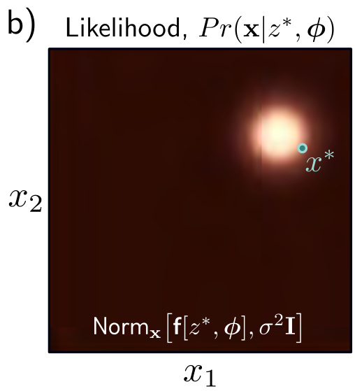
The likelihood \(Pr(x|z, \phi)\) is also normally distributed. Its mean is a nonlinear function \(f[z, \phi]\) of the latent variable, and its covariance \(\sigma^2 I\) is spherical:
\[Pr(x|z, \phi) = \text{Norm}_x\!\left[f[z, \phi], \sigma^2 I\right]. \tag{17.6}\]
The function \(f[z, \phi]\) is described by a deep network with parameters \(\phi\). This network is the decoder. The latent variable \(z\) is lower dimensional than the data \(x\). The model \(f[z,\phi]\) describes the important aspects of the data, and the remaining unmodelled aspects are ascribed to the noise \(\sigma^2 I\).
The data probability \(Pr(x|\phi)\) is found by marginalising over \(z\):
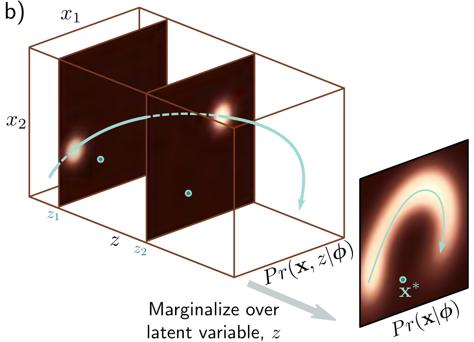
\[ \begin{aligned} Pr(x|\phi) &= \int Pr(x, z|\phi)\, dz \\ &= \int Pr(x|z, \phi) \cdot Pr(z)\, dz \\ &= \int \text{Norm}_x\!\left[f[z, \phi], \sigma^2 I\right] \cdot \text{Norm}_z[0, I]\, dz. \end{aligned} \tag{17.7} \]
This can be viewed as an infinite weighted sum — an infinite mixture — of spherical Gaussians with different means, where the weights are \(Pr(z)\) and the means are the network outputs \(f[z, \phi]\).
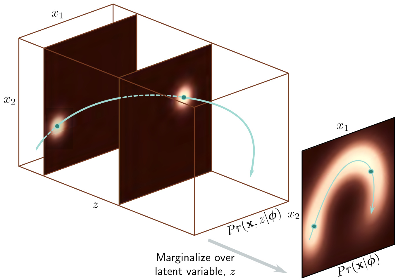
Notice what the figure shows. Every slice through the joint distribution at a fixed \(z\) is a plain spherical Gaussian. The means of those slices trace out a curved path through data space as \(z\) varies. Integrating over \(z\) smears the Gaussians along that path, and the result is a curved, multimodal, skewed density that no single Gaussian could represent. A one- or two-dimensional latent is already enough for this.
Generation
A new example \(x^*\) can be generated using ancestral sampling. We draw \(z^*\) from the prior \(Pr(z)\) and pass this through the network \(f[z^*, \phi]\) to compute the mean of the likelihood \(Pr(x|z^*, \phi)\), from which we draw \(x^*\). Both the prior and likelihood are normal distributions, so this is straightforward.
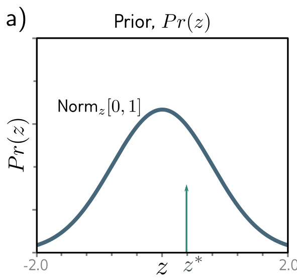
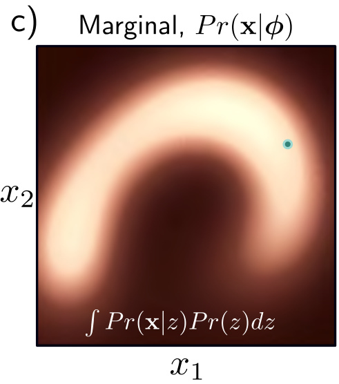
The sting is in the tail. Generation needs only one pass through the decoder, but evaluating \(Pr(x|\phi)\) requires the integral in equation 17.7, and there is no closed form for it. Sampling is easy; training is not.
Key ideas
- The prior is a plain standard normal. All the expressive power sits in the decoder \(f[z,\phi]\).
- The model is an infinite mixture of spherical Gaussians whose means lie on a manifold traced by the decoder.
- Ancestral sampling generates data in two draws and one forward pass.
- The marginal likelihood, which training needs, is the one thing the model cannot supply.
Learning outcomes
- nonlinear-latent-model Describe the continuous nonlinear latent variable model defined by a decoder network and sample from it.
Concepts
- latent-variable-models extends general latent variable models to continuous, multi-dimensional representations
- nonlinear-latent-variable-model defines the model in which the Gaussian likelihood mean is parameterised by a deep network \(f[z,\phi]\), and generated from by ancestral sampling
Intractable likelihood and the ELBO
To train the model, we maximise the log-likelihood over a training dataset \(\{x_i\}_{i=1}^{I}\) with respect to the model parameters. For simplicity we assume that the variance term \(\sigma^2\) in the likelihood expression is known, and concentrate on learning \(\phi\):
\[\hat\phi = \operatorname*{argmax}_{\phi}\left[\sum_{i=1}^{I} \log\!\left[Pr(x_i|\phi)\right]\right], \tag{17.8}\]
where
\[Pr(x_i|\phi) = \int \text{Norm}_{x_i}\!\left[f[z, \phi], \sigma^2 I\right] \cdot \text{Norm}_z[0, I]\, dz. \tag{17.9}\]
Prince states the difficulty plainly. This is intractable. There is no closed-form expression for the integral and no easy way to evaluate it for a particular value of \(x\).
To make progress, we define a lower bound on the log-likelihood. This is a function that is always less than or equal to the log-likelihood for a given value of \(\phi\), and will also depend on some other parameters \(\theta\). Eventually we will build a network to compute this lower bound and optimise it. To define it, we need Jensen’s inequality.
Jensen’s inequality
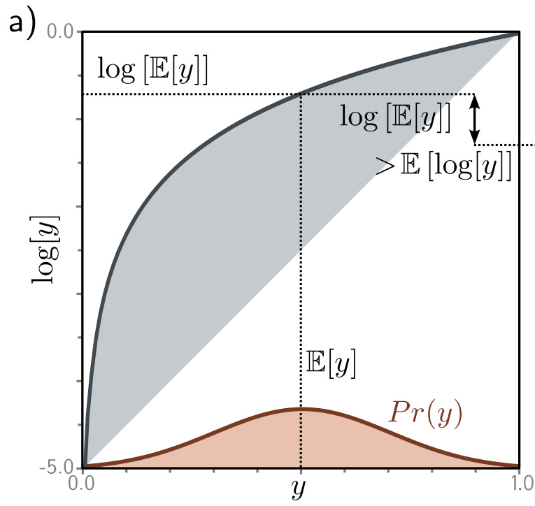
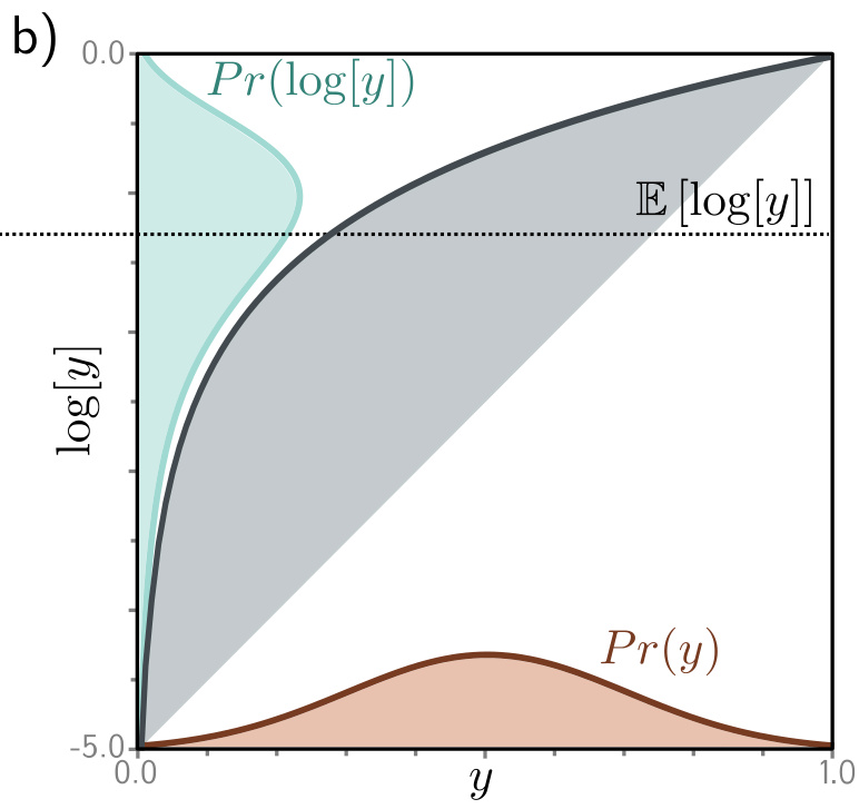
Jensen’s inequality says that a concave function \(g[\cdot]\) of the expectation of data \(y\) is greater than or equal to the expectation of the function of the data:
\[g\!\left[\mathbb{E}[y]\right] \ge \mathbb{E}\!\left[g[y]\right]. \tag{17.10}\]
In our case the concave function is the logarithm, so we have
\[\log\!\left[\mathbb{E}[y]\right] \ge \mathbb{E}\!\left[\log[y]\right], \tag{17.11}\]
or, writing out the expectation in full,
\[\log\!\left[\int Pr(y)\, y\, dy\right] \ge \int Pr(y) \log[y]\, dy. \tag{17.12}\]
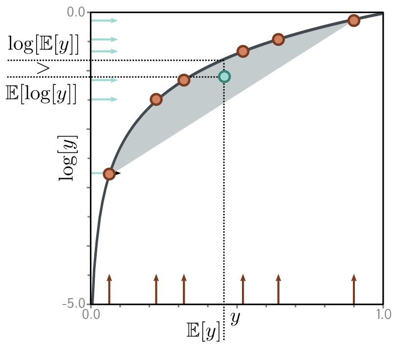
In fact the slightly more general statement is true:
\[\log\!\left[\int Pr(y)\, h[y]\, dy\right] \ge \int Pr(y) \log\!\left[h[y]\right] dy, \tag{17.13}\]
where \(h[y]\) is a function of \(y\). This follows because \(h[y]\) is another random variable with a new distribution. Since we never specified \(Pr(y)\), the relation remains true. Equation 17.13 is the form we will actually use.
Deriving the bound
We start by multiplying and dividing the log-likelihood by an arbitrary probability distribution \(q(z)\) over the latent variables:
\[ \begin{aligned} \log\!\left[Pr(x|\phi)\right] &= \log\!\left[\int Pr(x, z|\phi)\, dz\right] \\ &= \log\!\left[\int q(z)\, \frac{Pr(x, z|\phi)}{q(z)}\, dz\right]. \end{aligned} \tag{17.14} \]
We then use Jensen’s inequality for the logarithm, in the form of equation 17.13, with \(h[z] = Pr(x,z|\phi)/q(z)\):
\[\log\!\left[\int q(z)\, \frac{Pr(x, z|\phi)}{q(z)}\, dz\right] \ge \int q(z) \log\!\left[\frac{Pr(x, z|\phi)}{q(z)}\right] dz, \tag{17.15}\]
where the right-hand side is termed the evidence lower bound, or ELBO. It gets this name because \(Pr(x|\phi)\) is called the evidence in the context of Bayes’ rule.
In practice the distribution \(q(z)\) has parameters \(\theta\), so the ELBO can be written as
\[\text{ELBO}[\theta, \phi] = \int q(z|\theta) \log\!\left[\frac{Pr(x, z|\phi)}{q(z|\theta)}\right] dz. \tag{17.16}\]
To learn the nonlinear latent variable model, we maximise this quantity as a function of both \(\phi\) and \(\theta\). The neural architecture that computes this quantity is the VAE.
The bound holds for any \(q\). That freedom is what the next two sections spend: first on understanding what each of the two moves buys us, then on choosing a family of \(q\) we can compute with.
Learning outcomes
- derive-elbo Explain why maximum likelihood is intractable here and derive the evidence lower bound with Jensen’s inequality.
Concepts
- nonlinear-latent-variable-model demonstrates that evaluating the marginal log-likelihood for the continuous nonlinear latent model requires an intractable integral
- elbo defines the evidence lower bound as an optimisable surrogate for the intractable log-likelihood, and derives it from an auxiliary distribution \(q(z|\theta)\)
ELBO properties: tightness and reconstruction
The ELBO is a somewhat mysterious object when first encountered, so we now read the same expression two different ways.
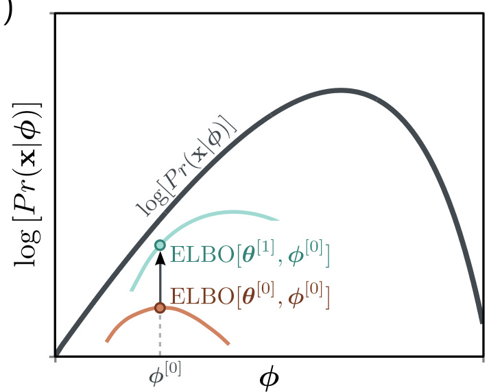
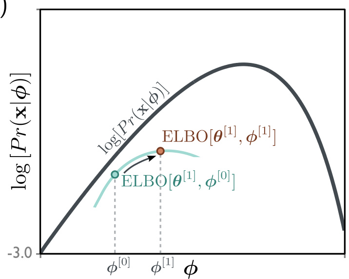
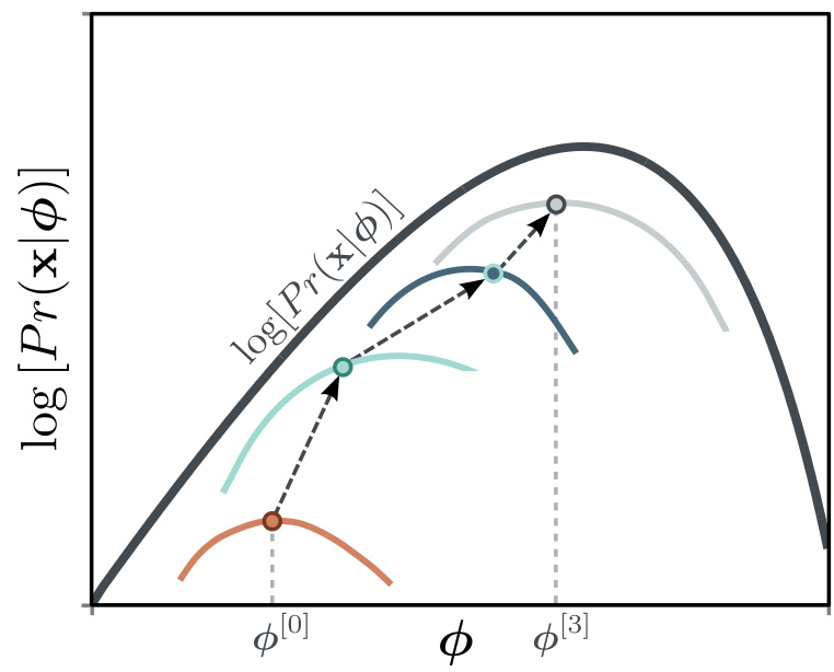
Consider that the original log-likelihood of the data is a function of the parameters \(\phi\), and that we want to find its maximum. For any fixed \(\theta\), the ELBO is still a function of \(\phi\), but one that must lie below the original likelihood function. When we change \(\theta\), we modify this function, and depending on our choice the lower bound may move closer to or further from the log-likelihood. When we change \(\phi\), we move along the lower bound function.
Tightness of the bound
The ELBO is tight when, for a fixed value of \(\phi\), the ELBO and the log-likelihood function coincide. To find the distribution \(q(z|\theta)\) that makes the bound tight, we factor the numerator of the log term using the definition of conditional probability:
\[ \begin{aligned} \text{ELBO}[\theta, \phi] &= \int q(z|\theta) \log\!\left[\frac{Pr(x, z|\phi)}{q(z|\theta)}\right] dz \\ &= \int q(z|\theta) \log\!\left[\frac{Pr(z|x, \phi) Pr(x|\phi)}{q(z|\theta)}\right] dz \\ &= \int q(z|\theta) \log\!\left[Pr(x|\phi)\right] dz + \int q(z|\theta) \log\!\left[\frac{Pr(z|x, \phi)}{q(z|\theta)}\right] dz \\ &= \log\!\left[Pr(x|\phi)\right] + \int q(z|\theta) \log\!\left[\frac{Pr(z|x, \phi)}{q(z|\theta)}\right] dz \\ &= \log\!\left[Pr(x|\phi)\right] - D_{KL}\!\left[q(z|\theta) \,\middle\|\, Pr(z|x, \phi)\right]. \end{aligned} \tag{17.17} \]
The first integral disappears between lines three and four because \(\log[Pr(x|\phi)]\) does not depend on \(z\), and the integral of the probability distribution \(q(z|\theta)\) is one. The last line is the definition of the KL divergence.
The KL divergence measures the “distance” between distributions and can only take non-negative values. It follows that the ELBO is a lower bound on \(\log[Pr(x|\phi)]\). The KL distance will be zero, and the bound will be tight, when \(q(z|\theta) = Pr(z|x, \phi)\). This is the posterior distribution over the latent variables \(z\) given observed data \(x\); it indicates which values of the latent variable could have been responsible for the data point.
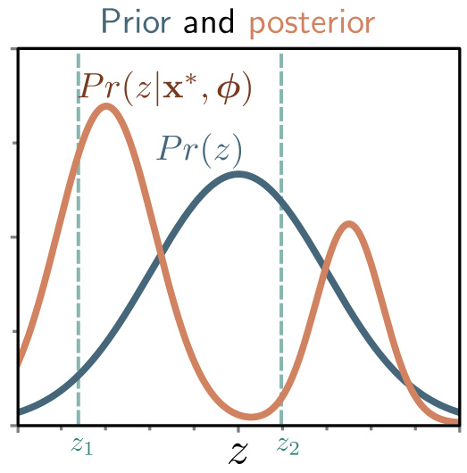
So the division of labour is exact. Optimising \(\theta\) improves the approximation and tightens the bound; optimising \(\phi\) improves the model itself.
ELBO as reconstruction loss minus KL distance to the prior
Equations 17.16 and 17.17 are two different ways to express the ELBO. A third way is to consider the bound as reconstruction error minus the distance to the prior:
\[ \begin{aligned} \text{ELBO}[\theta, \phi] &= \int q(z|\theta) \log\!\left[\frac{Pr(x, z|\phi)}{q(z|\theta)}\right] dz \\ &= \int q(z|\theta) \log\!\left[\frac{Pr(x|z, \phi) Pr(z)}{q(z|\theta)}\right] dz \\ &= \int q(z|\theta) \log\!\left[Pr(x|z, \phi)\right] dz + \int q(z|\theta) \log\!\left[\frac{Pr(z)}{q(z|\theta)}\right] dz \\ &= \int q(z|\theta) \log\!\left[Pr(x|z, \phi)\right] dz - D_{KL}\!\left[q(z|\theta) \,\middle\|\, Pr(z)\right], \end{aligned} \tag{17.18} \]
where the joint distribution \(Pr(x,z|\phi)\) has been factored into \(Pr(x|z,\phi)Pr(z)\) between the first and second lines, and the definition of KL divergence is used again in the last line.
In this formulation the first term measures the average agreement \(Pr(x|z, \phi)\) of the latent variable and the data. This measures the reconstruction accuracy. The second term measures the degree to which the auxiliary distribution \(q(z|\theta)\) matches the prior. This formulation is the one that is used in the variational autoencoder.
Equation 17.17 tells us how good the bound is: the slack is the KL divergence to the true posterior. Equation 17.18 tells us what to compute: a reconstruction term and a penalty against the prior. They are algebraically the same quantity.
Learning outcomes
- interpret-elbo Interpret the ELBO as reconstruction minus KL, and explain exactly when the bound is tight.
Concepts
- elbo shows that the gap between the ELBO and the log evidence is the KL divergence to the true posterior, and reformulates the bound as reconstruction minus KL distance to the prior
The variational approximation
We saw in equation 17.17 that the ELBO is tight when \(q(z|\theta)\) is the posterior \(Pr(z|x, \phi)\). In principle we can compute that posterior using Bayes’ rule:
\[Pr(z|x, \phi) = \frac{Pr(x|z, \phi) Pr(z)}{Pr(x|\phi)}, \tag{17.19}\]
but in practice this is intractable, because we cannot evaluate the evidence term \(Pr(x|\phi)\) in the denominator. That is the same integral that defeated maximum likelihood in the first place.
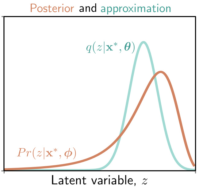
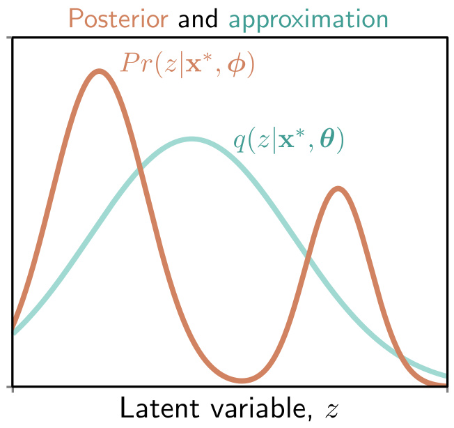
One solution is to make a variational approximation. We choose a simple parametric form for \(q(z|\theta)\) and use this to approximate the true posterior. Here we choose a multivariate normal distribution with mean \(\mu\) and diagonal covariance \(\Sigma\). This will not always match the posterior well, but will be better for some values of \(\mu\) and \(\Sigma\) than others. During training we will find the normal distribution that is “closest” to the true posterior \(Pr(z|x)\). This corresponds to minimising the KL divergence in equation 17.17, and moving the coloured ELBO curves upwards.
Amortising the approximation
The optimal choice for \(q(z|\theta)\) was the posterior \(Pr(z|x)\), and this depends on the data example \(x\). The variational approximation should do the same, so we choose
\[q(z|x, \theta) = \text{Norm}_z\!\left[g_\mu[x, \theta],\; g_\Sigma[x, \theta]\right], \tag{17.20}\]
where \(g[x, \theta]\) is a second neural network with parameters \(\theta\) that predicts the mean \(\mu\) and variance \(\Sigma\) of the normal variational approximation.
This is the step worth pausing on. Every data point \(x_i\) has its own best \(q\), and the naive reading of equation 17.16 would have us optimise a separate pair \((\mu_i, \Sigma_i)\) for every training example. Instead one network answers for all of them. This is amortisation: the cost of inference is paid once, in the weights \(\theta\), and reused for every example including ones never seen in training.
Two consequences follow.
The Gaussian family is a restriction, and it costs us tightness.
The residual \(D_{KL}[q(z|x,\theta) \| Pr(z|x,\phi)]\) never reaches zero when the true posterior is multi-modal.
Diagonal covariance makes both the sampling step and the KL term to \(\text{Norm}[0,I]\) available in closed form.
That is what makes the loss of the next section computable at all.
Naming matters here. The network \(g[x, \theta]\) is the encoder, and it exists to serve training. The generative model of the previous sections does not contain it.
Learning outcomes
- variational-approximation Explain the encoder as an amortised variational approximation to the true posterior.
Concepts
- variational-approximation specifies the data-conditioned Gaussian approximation \(q(z|x,\theta) = \text{Norm}_z[g_\mu[x,\theta], g_\Sigma[x,\theta]]\) computed by an encoder network
The VAE architecture and algorithm
Finally we can describe the VAE. We build a network that computes the ELBO, using the reconstruction-minus-KL form of equation 17.18 with the amortised approximation of equation 17.20:
\[\text{ELBO}[\theta, \phi] = \int q(z|x, \theta) \log\!\left[Pr(x|z, \phi)\right] dz - D_{KL}\!\left[q(z|x, \theta) \,\middle\|\, Pr(z)\right]. \tag{17.21}\]
The first term still involves an intractable integral, but since it is an expectation with respect to \(q(z|x, \theta)\), we can approximate it by sampling. For any function \(\text{a}[\cdot]\) we have
\[\mathbb{E}_z\!\left[\text{a}[z]\right] = \int \text{a}[z]\, q(z|x, \theta)\, dz \approx \frac{1}{N} \sum_{n=1}^{N} \text{a}[z_n^*], \tag{17.22}\]
where \(z_n^*\) is the \(n^{\text{th}}\) sample from \(q(z|x, \theta)\). This is known as a Monte Carlo estimate. For a very approximate estimate, we can just use a single sample \(z^*\) from \(q(z|x, \theta)\):
\[\text{ELBO}[\theta, \phi] \approx \log\!\left[Pr(x|z^*, \phi)\right] - D_{KL}\!\left[q(z|x, \theta) \,\middle\|\, Pr(z)\right]. \tag{17.23}\]
The second term is the KL divergence between the variational distribution \(q(z|x,\theta) = \text{Norm}_z[\mu, \Sigma]\) and the prior \(Pr(z) = \text{Norm}_z[0,I]\). The KL divergence between two normal distributions can be calculated in closed form. For the special case where one distribution has parameters \(\mu, \Sigma\) and the other is a standard normal, it is given by
\[D_{KL}\!\left[q(z|x, \theta) \,\middle\|\, Pr(z)\right] = \frac{1}{2}\left(\text{Tr}[\Sigma] + \mu^{T}\mu - D_z - \log\!\left[\det[\Sigma]\right]\right), \tag{17.24}\]
where \(D_z\) is the dimensionality of the latent space. Note what this buys: the regularisation term contributes an exact, differentiable penalty with no sampling noise at all. Only the reconstruction term is estimated.
The VAE algorithm
To summarise, we aim to build a model that computes the evidence lower bound for a point \(x\). Then we use an optimisation algorithm to maximise this lower bound over the dataset and hence improve the log-likelihood. To compute the ELBO we:
- compute the mean \(\mu\) and variance \(\Sigma\) of the variational posterior distribution \(q(z|\theta, x)\) for this data point \(x\) using the network \(g[x, \theta]\),
- draw a sample \(z^*\) from this distribution, and
- compute the ELBO using equation 17.23.
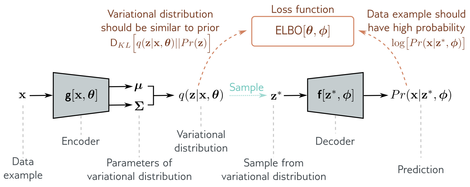
It should now be clear why this is called a variational autoencoder. It is variational because it computes a Gaussian approximation to the posterior distribution. It is an autoencoder because it starts with a data point \(x\), computes a lower-dimensional latent vector \(z\) from this, and then uses this vector to recreate the data point \(x\) as closely as possible. In this context the mapping from the data to the latent variable by the network \(g[x, \theta]\) is called the encoder, and the mapping from the latent variable to the data by the network \(f[z, \phi]\) is called the decoder.
The VAE computes the ELBO as a function of both \(\phi\) and \(\theta\). To maximise this bound, we run mini-batches of samples through the network and update these parameters with an optimisation algorithm such as SGD or Adam. The gradients of the ELBO with respect to the parameters are computed as usual using automatic differentiation. During this process we are both moving between the coloured curves (changing \(\theta\)) and along them (changing \(\phi\)). The parameters \(\phi\) change to assign the data a higher likelihood in the nonlinear latent variable model.
The list above contains a sampling operation between the encoder and the decoder. Automatic differentiation cannot pass a gradient through it, so as written the encoder parameters \(\theta\) would never be updated. The next section repairs this.
Learning outcomes
- vae-algorithm Assemble encoder and decoder into a VAE and write down its training algorithm and loss.
Concepts
- variational-autoencoder assembles the encoder \(g[x,\theta]\) and decoder \(f[z,\phi]\) into the architecture that optimises the single-sample ELBO estimate by mini-batch SGD or Adam
- elbo is evaluated inside the network as a closed-form Gaussian KL term plus a Monte Carlo reconstruction term
- variational-approximation supplies the intermediate distribution \(q(z|x,\theta)\) from which the latent vector is sampled
The reparameterization trick
There is one more complication. The network involves a sampling step, and it is difficult to differentiate through this stochastic component. However, differentiating past this step is necessary to update the parameters \(\theta\) that precede it in the network.
The reason is worth stating precisely. The encoder produces \(\mu\) and \(\Sigma\); the sample \(z^*\) is then drawn from \(\text{Norm}_z[\mu, \Sigma]\). A draw is not a function of \(\mu\) and \(\Sigma\) in the sense backpropagation requires — there is no derivative \(\partial z^* / \partial \mu\) for a sampling operation. The chain rule stops at that node, and everything upstream of it, which is the whole encoder, receives no gradient.
Fortunately there is a simple solution. We can move the stochastic part into a branch of the network that draws a sample \(\epsilon^*\) from \(\text{Norm}_\epsilon[0, I]\), and then use the relation
\[z^* = \mu + \Sigma^{1/2}\epsilon^*, \tag{17.25}\]
to draw from the intended Gaussian. Now we can compute the derivatives as usual, because the backpropagation algorithm does not need to pass down the stochastic branch. This is known as the reparameterization trick.
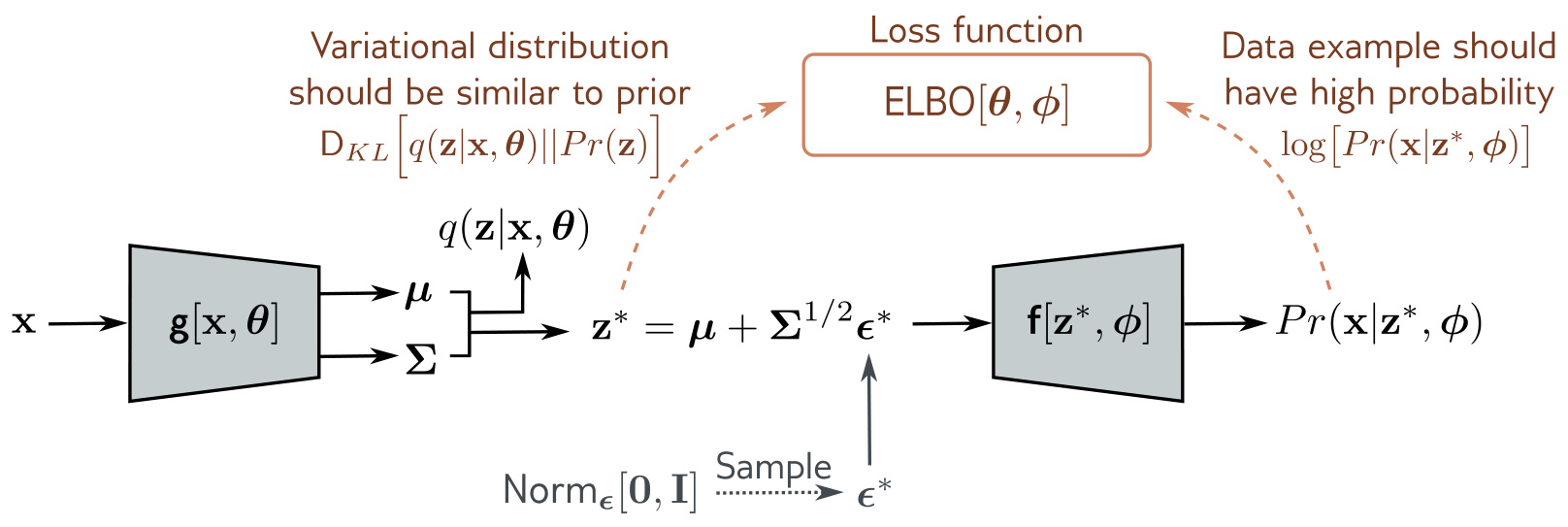
Trace the gradient path through the reparameterised graph and the fix is transparent.
\(\epsilon^*\) enters the graph as an input, on a branch with no parameters at all.
Nothing upstream of it needs a gradient, so nothing is lost by not having one.
Given \(\epsilon^*\), the expression \(\mu + \Sigma^{1/2}\epsilon^*\) is an ordinary affine function of \(\mu\) and \(\Sigma\).
Its derivatives are \(I\) and a term in \(\epsilon^*\) respectively, both perfectly well defined.
The distribution of \(z^*\) is unchanged.
Shifting standard normal noise by \(\mu\) and scaling it by \(\Sigma^{1/2}\) produces exactly \(\text{Norm}_z[\mu, \Sigma]\), which is what equation 17.22 sampled.
With this in place, the whole VAE trains end to end with ordinary automatic differentiation. Both factors that determine the lower bound are updated at each iteration: the decoder parameters \(\phi\) and the encoder parameters \(\theta\).
The reparameterization trick is one way to differentiate an expectation whose distribution depends on the parameters. Prince notes there are alternatives — the score function estimator, discussed in the closing section — but that the reparameterization trick usually gives an estimator with low variance.
Learning outcomes
- reparameterization-trick Apply the reparameterization trick to backpropagate through a stochastic latent layer.
- vae-algorithm Assemble encoder and decoder into a VAE and write down its training algorithm and loss.
Concepts
- reparameterization-trick rewrites the latent sample as \(z^* = \mu + \Sigma^{1/2}\epsilon^*\) so that gradients from the ELBO loss reach the encoder parameters \(\theta\)
Applications of trained VAEs
Variational autoencoders have many uses, including denoising, anomaly detection, and compression. We look here at four things a trained model gives us, all for image data.
Approximating sample probability
We argued in the training section that it is not possible to evaluate the probability of a sample with the VAE, which describes this probability as
\[ \begin{aligned} Pr(x) &= \int Pr(x|z) Pr(z)\, dz = \mathbb{E}_z\!\left[Pr(x|z)\right] = \mathbb{E}_z\!\left[\text{Norm}_x[f[z, \phi], \sigma^2 I]\right]. \end{aligned} \tag{17.26} \]
In principle we could approximate this by drawing samples from \(Pr(z) = \text{Norm}_z[0,I]\) and computing
\[Pr(x) \approx \frac{1}{N}\sum_{n=1}^{N} Pr(x|z_n). \tag{17.27}\]
However, the curse of dimensionality means that almost all values of \(z_n\) that we draw would have a very low probability \(Pr(x|z_n)\); we would have to draw an enormous number of samples to get a reliable estimate.
A better approach is importance sampling. We sample \(z\) from an auxiliary distribution \(q(z)\), evaluate \(Pr(x|z_n)\), and rescale the resulting values by the probability \(q(z)\) under the new distribution:
\[ \begin{aligned} Pr(x) &= \int Pr(x|z) Pr(z)\, dz = \int \frac{Pr(x|z)Pr(z)}{q(z)} q(z)\, dz \\ &= \mathbb{E}_{q(z)}\!\left[\frac{Pr(x|z)Pr(z)}{q(z)}\right] \approx \frac{1}{N}\sum_{n=1}^{N} \frac{Pr(x|z_n)Pr(z_n)}{q(z_n)}. \end{aligned} \tag{17.28} \]
If \(q(z)\) is close to the region of \(z\) where \(Pr(x|z)\) has high likelihood, we focus the sampling on the relevant area of space and estimate \(Pr(x)\) much more efficiently. The product \(Pr(x|z)Pr(z)\) we are trying to integrate is proportional to the posterior \(Pr(z|x)\) by Bayes’ rule. Hence a sensible choice of auxiliary distribution \(q(z)\) is the variational posterior \(q(z|x)\) computed by the encoder.
With sufficient samples this provides a better estimate than the lower bound, and could be used to evaluate the quality of the model by evaluating the log-likelihood of test data. Alternatively, it could be used as a criterion for determining whether new examples belong to the distribution or are anomalous.
Generation
VAEs build a probabilistic model, and it is easy to sample from this model by drawing from the prior \(Pr(z)\), passing the result through the decoder \(f[z, \phi]\), and adding noise according to \(Pr(x|f[z, \phi])\). Unfortunately, samples from vanilla VAEs are generally low-quality. This is partly because of the naïve spherical Gaussian noise model and partly because of the Gaussian models used for the prior and variational posterior.
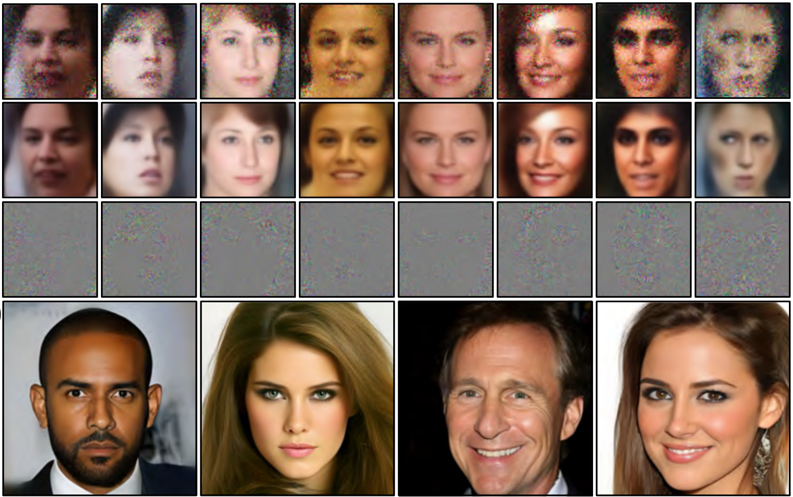
One trick to improve generation quality is to sample from the aggregated posterior \(q(z|\theta) = (1/I)\sum_i q(z|x_i, \theta)\) rather than the prior. This is the average posterior over all samples, and is a mixture of Gaussians that is more representative of the true distribution in latent space. Modern VAEs can produce high-quality samples, but only by using hierarchical priors and specialised network architecture and regularisation techniques.
Resynthesis
VAEs can also be used to modify real data. A data point \(x\) can be projected into the latent space either by (i) taking the mean of the distribution predicted by the encoder, or (ii) by using an optimisation procedure to find the latent variable \(z\) that maximises the posterior, which Bayes’ rule tells us is proportional to \(Pr(x|z)Pr(z)\).
Suppose multiple images labelled as “neutral” or “smiling” are projected into latent space. The vector representing this change is estimated by taking the difference in latent space between the means of these two groups. A second vector is estimated to represent “mouth closed” versus “mouth open”.
Now the image of interest is projected into the latent space, and the representation is modified by adding or subtracting these vectors. To generate intermediate images, spherical linear interpolation, or Slerp, is used rather than linear interpolation. In 3D this would be the difference between interpolating along the surface of a sphere versus digging a straight tunnel through its body.
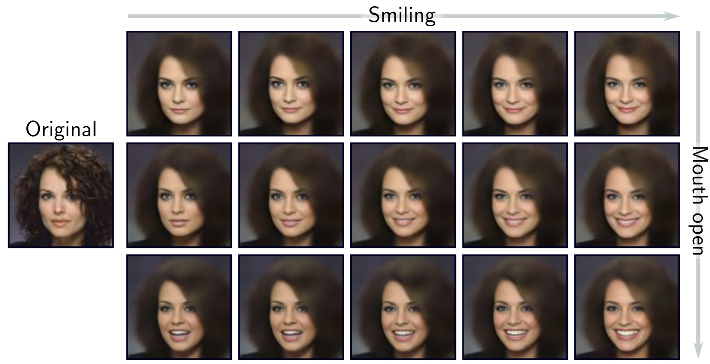
The process of encoding, possibly modifying, and decoding again is known as resynthesis. It can also be done with GANs and normalizing flows. However, in GANs there is no encoder, so a separate procedure must be used to find the latent variable that corresponds to the observed data.
Learning outcomes
- vae-applications Use a trained VAE to generate, to estimate sample probability, and to resynthesise data.
Concepts
- variational-approximation serves as the proposal distribution in the importance sampling estimate of the true data likelihood \(Pr(x)\)
- variational-autoencoder generates samples from its prior, with quality limited in the vanilla model and improved by hierarchical latent spaces
- resynthesis encodes real data, moves along latent attribute directions, and decodes again, using spherical linear interpolation for intermediates
Disentanglement and failure modes
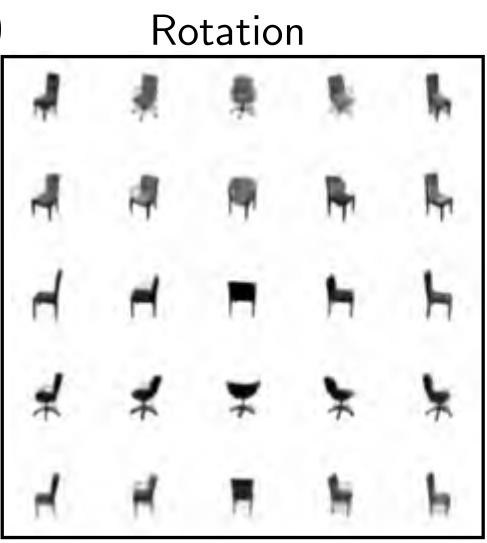
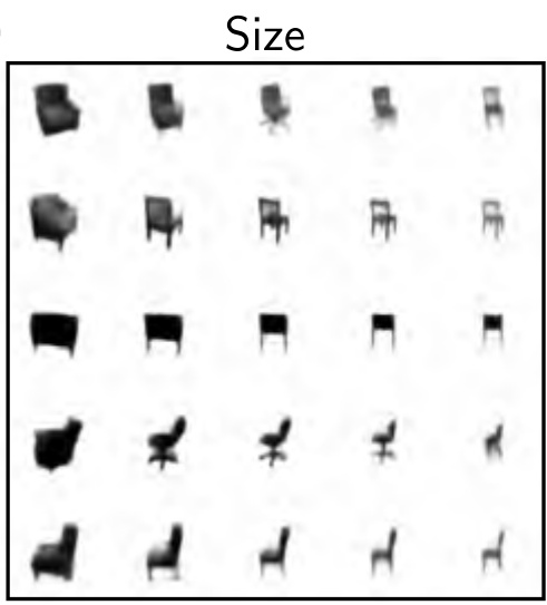
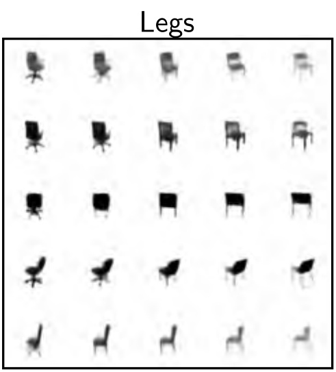
In the resynthesis example above, the directions in space representing interpretable properties had to be estimated using labelled training data. Other work attempts to improve the characteristics of the latent space itself, so that its coordinate directions correspond to real-world properties. When each dimension represents an independent real-world factor, the latent space is described as disentangled. For face images, we might hope to uncover head pose or hair colour as independent factors.
Reshaping the loss
Methods to encourage disentanglement typically add regularisation terms to the loss function, based on either the posterior \(q(z|x, \theta)\) over the latent variables, or the aggregated posterior \(q(z|\theta) = (1/I)\sum_i q(z|x_i, \theta)\):
\[L_{\text{new}} = -\text{ELBO}[\theta, \phi] + \lambda_1 \mathbb{E}_{Pr(x)}\!\left[\text{r}_1\!\left[q(z|x, \theta)\right]\right] + \lambda_2\, \text{r}_2\!\left[q(z|\theta)\right]. \tag{17.29}\]
Here the regularisation term \(\text{r}_1[\cdot]\) is a function of the posterior and is weighted by \(\lambda_1\). The term \(\text{r}_2[\cdot]\) is a function of the aggregated posterior and is weighted by \(\lambda_2\).
For example, the beta VAE upweights the second term in the ELBO of equation 17.18:
\[\text{ELBO}[\theta, \phi] \approx \log\!\left[Pr(x|z^*, \phi)\right] - \beta \cdot D_{KL}\!\left[q(z|x, \theta) \,\middle\|\, Pr(z)\right], \tag{17.30}\]
where \(\beta > 1\) determines how much more deviation from the prior \(Pr(z)\) is weighted relative to the reconstruction error. Since the prior is usually a multivariate normal with a spherical covariance matrix, its dimensions are independent. Hence, up-weighting this term encourages the posterior distributions to be less correlated. Another variant is the total correlation VAE, which adds a term to decrease the total correlation between variables in the latent space and maximises the mutual information between a small subset of the latent variables and the observations.
Failure modes
Prince’s chapter notes are candid about what the basic model gets wrong.
Blurry reconstructions. Zhao et al. (2017c) provide evidence that the blurry reconstructions are partly due to Gaussian noise and also because of the sub-optimal posterior distributions induced by the variational approximation.
Some of the best synthesis results have come from using a discrete latent space modelled by a sophisticated autoregressive model, or from using hierarchical latent spaces.
Posterior collapse. One potential problem in training is posterior collapse, in which the encoder always predicts the prior distribution.
It was identified by Bowman et al. (2015) and can be mitigated by gradually increasing the term that encourages the KL distance between the posterior and the prior to be small during training.
The information preference problem. Chen et al. (2017) noted that when more complex likelihood terms are used, such as the PixelCNN, the output can cease to depend on the latent variables at all.
This was addressed in the InfoVAE by adding an extra term that maximised the mutual information between the latent and observed distributions.
Holes in the latent space. There can be regions of latent space that do not correspond to any realistic sample.
Xu et al. (2020) introduce the constrained posterior VAE, which adds a regularisation term to prevent these vacant regions and allows better interpolation from real samples.
Learning outcomes
- disentanglement-and-limits Modify the VAE loss for disentangled latents, and name the failure modes of the basic model.
Concepts
- disentanglement reviews loss modifications such as the beta VAE and the total correlation VAE that penalise latent dependency to isolate independent semantic factors
- posterior-collapse names the failure in which the encoder ignores its input and predicts the prior, and the KL-annealing and architectural remedies for it
- reparameterization-trick is compared with the alternative score function estimator, which has higher variance
Closing: towards diffusion models
Prince’s own summary is short, and worth reading against what we have built.
The VAE is an architecture that helps to learn a nonlinear latent variable model over \(x\). This model can generate new examples by sampling from the latent variable, passing the result through a deep network, and then adding independent Gaussian noise. It is not possible to compute the likelihood of a data point in closed form, and this poses problems for training with maximum likelihood. However, we can define a lower bound on the likelihood and maximise this bound. Unfortunately, for the bound to be tight, we need to compute the posterior probability of the latent variable given the observed data, which is also intractable. The solution is to make a variational approximation. This is a simpler distribution, usually a Gaussian, that approximates the posterior and whose parameters are computed by a second encoder network.
What you can now do
A latent variable model describes \(Pr(x)\) by marginalising a joint distribution over an unobserved \(z\).
A simple prior and a simple conditional compose into a complex marginal — first as a finite mixture of Gaussians, then as an infinite one.
The marginal likelihood of the nonlinear latent variable model has no closed form, so maximum likelihood is out of reach.
Sampling from the model and scoring a point under it are not equally hard. Generation was never the problem.
Jensen’s inequality converts \(\log \mathbb{E}[\cdot]\) into \(\mathbb{E}[\log \cdot]\) and yields the ELBO.
The inequality holds for any \(q\), which is exactly the freedom that makes an encoder network admissible.
The ELBO reads two ways: log-likelihood minus KL to the true posterior, and reconstruction minus KL to the prior.
The first says how tight the bound is; the second says what code to write.
An encoder network amortises the variational approximation across all data points.
One set of weights replaces a separate optimisation for every training example, and generalises to examples never seen.
The reparameterization trick moves the randomness onto a parameter-free input branch.
\(z^* = \mu + \Sigma^{1/2}\epsilon^*\) has the same distribution as the original draw, but is differentiable in \(\mu\) and \(\Sigma\).
A trained model generates, scores by importance sampling, resynthesises, and can be pushed towards disentangled latents.
Each of these is a use of the latent space, not of the training architecture.
Where this goes next
The next unit is Chapter 18: Diffusion models. Prince closes chapter 17 by pointing directly at it. To create high-quality samples from the VAE, it seems to be necessary to model the latent space with more sophisticated probability distributions than the Gaussian prior and posterior. One option is to use hierarchical priors, in which one latent variable generates another. The next chapter discusses diffusion models, which produce very high-quality examples and can be viewed as hierarchical VAEs.
Read that framing carefully, because it means everything in this unit carries over. Diffusion models are latent variable models, they are trained by maximising a lower bound of the same kind, and their latent variables are reparameterised Gaussians. What changes is the choice of \(q\).
Learning outcomes
- latent-variable-models Explain how a latent variable model describes a complex density by marginalising a joint distribution.
- nonlinear-latent-model Describe the continuous nonlinear latent variable model defined by a decoder network and sample from it.
- derive-elbo Explain why maximum likelihood is intractable here and derive the evidence lower bound with Jensen’s inequality.
- interpret-elbo Interpret the ELBO as reconstruction minus KL, and explain exactly when the bound is tight.
- variational-approximation Explain the encoder as an amortised variational approximation to the true posterior.
- vae-algorithm Assemble encoder and decoder into a VAE and write down its training algorithm and loss.
- reparameterization-trick Apply the reparameterization trick to backpropagate through a stochastic latent layer.
- vae-applications Use a trained VAE to generate, to estimate sample probability, and to resynthesise data.
- disentanglement-and-limits Modify the VAE loss for disentangled latents, and name the failure modes of the basic model.
Concepts
- variational-autoencoder recaps how the encoder-decoder pair, the ELBO and the reparameterization trick together optimise a nonlinear latent variable model
- nonlinear-latent-variable-model reiterates the core structure of the generative model the VAE exists to train
References
- Understanding Deep Learning, Simon Prince, 2026 — Link — Page 341-362