Lecture notes — Chapter 18: Diffusion models
ver. 1.0.0, chapter_18_diffusion_models
← Chapter 18: Diffusion models
ver. 1.0.0 · 2026-08-22 10:24:13
Where we are
In Chapter 17: Variational autoencoders we fitted a latent variable model by maximising an evidence lower bound. The encoder \(q(z|x)\) was a learned Gaussian, the decoder was a network, and the bound was tight exactly when the encoder matched the true posterior. We paid for that with a learned encoder that could collapse, and with samples that were often blurry.
This unit keeps the bound and discards the learned encoder. In its place we put a fixed procedure: add a little Gaussian noise, \(T\) times over, until nothing but noise remains. Nothing in that direction is learned. What we learn is the reverse — a network trained to undo one noising step. Prince notes the family relation directly: diffusion models can be thought of as a special case of a hierarchical variational autoencoder in which the encoder is fixed and the latent space has the same size as the data.
Two properties of this design deserve stating before we begin. The latent variables \(z_1, \dots, z_T\) have the same dimension as \(x\), so there is no bottleneck to squeeze information through. And because the encoder has no parameters, the decoder must do all the work of making the bound tight.
The chapter assumes familiarity with variational autoencoders. If the ELBO, Jensen’s inequality or the reparameterization trick are not yet comfortable, return to Chapter 17 first.
What you will be able to do
forward-process— Describe the fixed forward noising process and the role of the variance schedule.diffusion-kernel— Use the closed-form diffusion kernel to jump to any noise level in one step.reverse-process— Define the learned reverse process and relate it to the tractable conditional \(q(z_{t-1}|z_t, x)\).diffusion-elbo— Derive the diffusion ELBO and simplify it into a sum of per-timestep KL terms.noise-prediction-loss— Reparameterize target and network to obtain the simple noise-prediction loss.training-and-sampling-loops— Write the training loop and the ancestral sampling loop for a diffusion model.image-implementation— Explain how a diffusion model is implemented for images with a time-conditioned U-Net.faster-sampling— Accelerate sampling with deterministic and step-skipping formulations.conditioning-and-scaling— Condition generation on class or text and scale to high resolution with cascades.
What we will cover
- Diffusion model — a generative model pairing a prespecified stochastic encoder with a learned stochastic decoder.
- Forward (diffusion) process — the fixed Markov chain that blends data with white noise over \(T\) steps.
- Noise schedule — the hyperparameters \(\beta_1 \dots \beta_T\) that set how fast the blending proceeds.
- Diffusion kernel — the closed-form \(q(z_t|x)\) that lets us reach any timestep in one operation.
- Reverse (decoder) process — the learned chain of Gaussian mappings from \(z_T\) back to \(x\).
- Evidence lower bound for diffusion — the variational objective, which reduces to per-step KL divergences.
- Noise prediction reparameterization — the rewriting that turns that objective into a plain squared error on \(\epsilon\).
- Denoising diffusion implicit models (DDIM) — a deterministic, non-Markovian variant that permits step skipping.
- Classifier guidance — steering the reverse update with the gradient of a noise-aware classifier.
- Classifier-free guidance — conditioning the denoising network directly and dropping the condition during training.
- Cascaded diffusion models — a pipeline of models that generates small and super-resolves.
From variational autoencoders to diffusion models
Let us fix the shape of the model before touching any algebra. A diffusion model consists of an encoder and a decoder. The encoder takes a data sample \(x\) and maps it through a series of intermediate latent variables \(z_1 \dots z_T\). The decoder reverses this; it starts with \(z_T\) and maps back through \(z_{T-1}, \dots, z_1\) until it finally re-creates a data point \(x\). In both directions the mappings are stochastic rather than deterministic.
The difference from Chapter 17 is where the parameters live.
The encoder is prespecified. It gradually blends the input with samples of white noise. Since this process is prespecified, all the learned parameters are in the decoder.
There is no encoder network to train, and therefore no posterior collapse to guard against.
With enough steps, the conditional distribution \(q(z_T|x)\) and the marginal distribution \(q(z_T)\) of the final latent variable both become the standard normal distribution.
That is the distribution we will start sampling from at generation time, so it must be one we can draw from trivially.
In the decoder, a series of networks are trained to map backward between each adjacent pair of latent variables \(z_t\) and \(z_{t-1}\). The loss function encourages each network to invert the corresponding encoder step.
Noise is gradually removed from the representation until a realistic-looking data example remains.
To generate a new data example \(x\), we draw a sample from \(q(z_T)\) and pass it through the decoder.
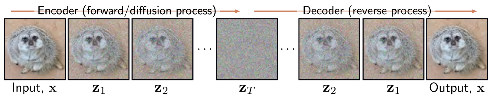
It is worth placing diffusion models among their neighbours, as Prince does at the head of the chapter. Generative adversarial models produce plausible samples but do not define a probability distribution over the data. Normalizing flows do define such a distribution but must constrain every layer to be invertible with an easily computed Jacobian determinant. Variational autoencoders have a solid probabilistic foundation, but the likelihood is intractable and must be approximated by a lower bound. Diffusion models resemble normalizing flows in mapping latent variables to data of the same dimension, and resemble variational autoencoders in bounding the likelihood — but their encoder is predetermined, and the goal is to learn a decoder that inverts it.
The forward or diffusion process runs from data to noise. This is the opposite nomenclature to normalizing flows, where the inverse mapping moves from the data to the latent variable and the forward mapping moves back again.
The remainder of the unit follows the chapter’s own order. We examine the encoder in detail, because its properties are non-obvious but critical for the learning algorithm. We then define the decoder, derive the training objective, reformulate it into something practical, and finish with implementation.
Learning outcomes
- forward-process Describe the fixed forward noising process and the role of the variance schedule.
- reverse-process Define the learned reverse process and relate it to the tractable conditional \(q(z_{t-1}|z_t, x)\).
- diffusion-elbo Derive the diffusion ELBO and simplify it into a sum of per-timestep KL terms.
The forward process and its noise schedule
The forward (diffusion) process maps a data example \(x\) through a series of intermediate variables \(z_1, z_2, \dots, z_T\) of the same size as \(x\), according to
\[ \begin{aligned} z_1 &= \sqrt{1-\beta_1}\cdot x + \sqrt{\beta_1}\cdot \epsilon_1 \\ z_t &= \sqrt{1-\beta_t}\cdot z_{t-1} + \sqrt{\beta_t}\cdot \epsilon_t \qquad \forall\, t \in 2, \dots, T, \end{aligned} \]
where \(\epsilon_t\) is noise drawn from a standard normal distribution.
Read the update as two operations in one line. The first term attenuates the data plus any noise added so far, and the second adds more noise. The attenuation is what keeps the variance from growing without bound: shrinking by \(\sqrt{1-\beta_t}\) removes exactly as much variance as adding noise of variance \(\beta_t\) puts back.
The hyperparameters \(\beta_t \in [0,1]\) determine how quickly the noise is blended and are collectively known as the noise schedule. Equivalently, in probabilistic form,
\[ \begin{aligned} q(z_1|x) &= \text{Norm}_{z_1}\!\left[\sqrt{1-\beta_1}\,x,\; \beta_1 I\right] \\ q(z_t|z_{t-1}) &= \text{Norm}_{z_t}\!\left[\sqrt{1-\beta_t}\,z_{t-1},\; \beta_t I\right] \qquad \forall\, t \in \{2,\dots,T\}. \end{aligned} \]
Each conditional is a normal distribution with a mean slightly closer to zero than the current point, and a fixed variance \(\beta_t\).
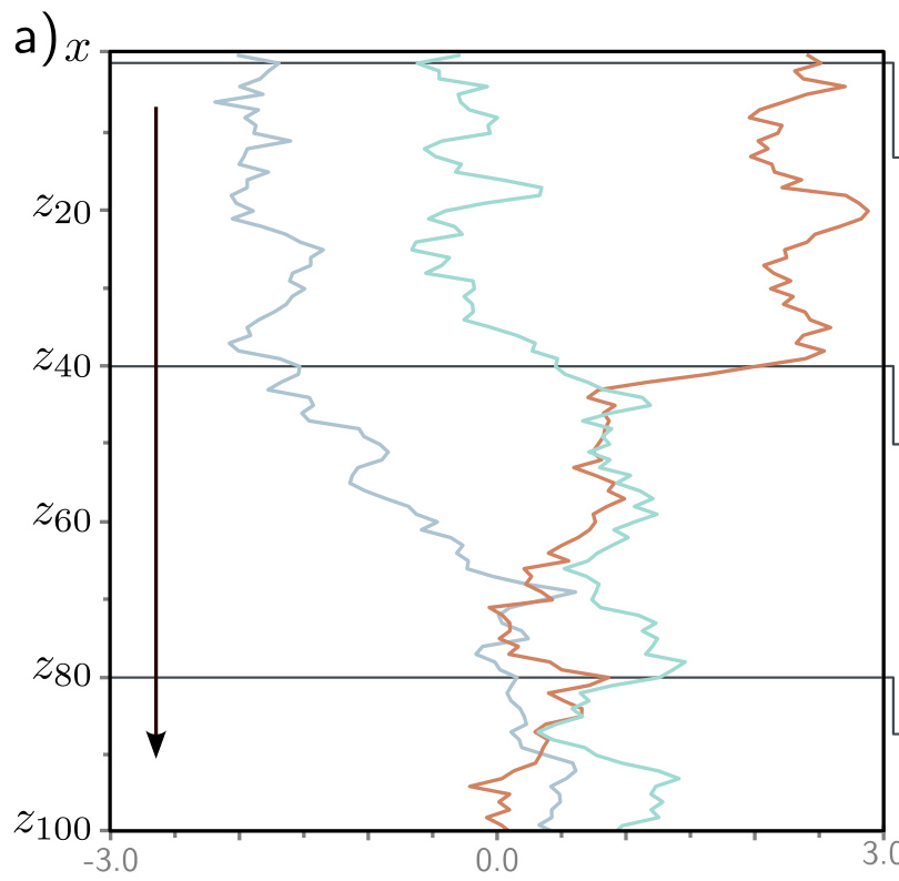
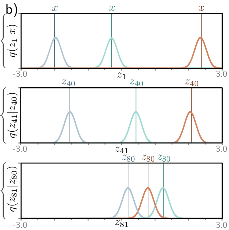
This is a Markov chain, because the probability of \(z_t\) is determined entirely by the value of the immediately preceding variable \(z_{t-1}\). With sufficient steps \(T\), all traces of the original data are removed, and \(q(z_T|x) = q(z_T)\) becomes a standard normal distribution. The joint distribution of all the latent variables given \(x\) therefore factorises:
\[ q(z_{1\dots T}|x) = q(z_1|x)\prod_{t=2}^{T} q(z_t|z_{t-1}). \]
Notice what is absent. There are no parameters anywhere in these equations. Contrast the variational autoencoder, whose encoder was a network with weights to be fitted and a posterior that could collapse onto the prior. Here the only design decision is \(\{\beta_t\}\), and it is a hyperparameter, not a learned quantity.
Prince writes \(q(z_t|z_{t-1})\) rather than \(Pr(z_t|z_{t-1})\) to match the notation used for the VAE encoder in the previous chapter. The letter \(q\) marks a distribution belonging to the encoder side.
The choice of schedule matters for a reason we will meet twice more. Small \(\beta_t\) keeps each step gentle, which is what makes the true reverse step close to Gaussian and therefore modellable. Small \(\beta_t\) also means many steps are needed before the data is destroyed. The tension between those two facts is the source of the sampling cost we address later.
Learning outcomes
- forward-process Describe the fixed forward noising process and the role of the variance schedule.
Concepts
- diffusion-model defines diffusion models as a prespecified stochastic encoder plus a learned reverse decoder
- forward-process presents the explicit equations for the forward Markov transitions \(q(z_t|z_{t-1})\)
- reverse-process describes how the decoder inverts the forward mapping step by step to recover data
- noise-schedule introduces the parameters \(\beta_t \in [0,1]\) as the schedule regulating noise addition
The diffusion kernel and the marginals
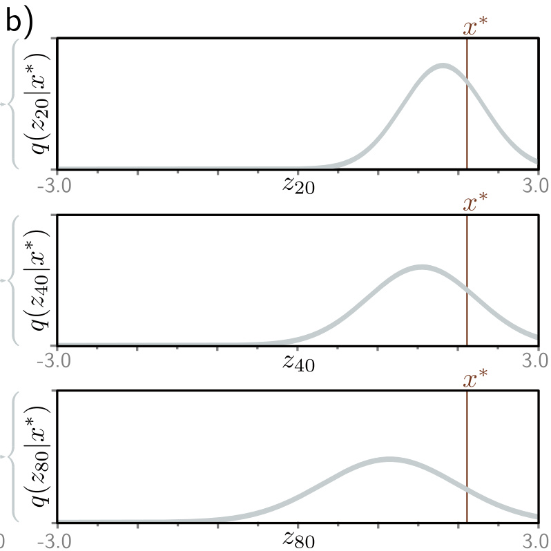
To train the decoder to invert the forward process, we need multiple samples \(z_t\) at time \(t\) for the same example \(x\). Generating these sequentially is time-consuming when \(t\) is large. Fortunately there is a closed-form expression for \(q(z_t|x)\), which lets us draw \(z_t\) directly without computing \(z_1 \dots z_{t-1}\). This is the diffusion kernel.
Deriving it
Take the first two steps and substitute the first into the second:
\[ \begin{aligned} z_2 &= \sqrt{1-\beta_2}\left(\sqrt{1-\beta_1}\cdot x + \sqrt{\beta_1}\cdot\epsilon_1\right) + \sqrt{\beta_2}\cdot\epsilon_2 \\ &= \sqrt{1-\beta_2}\sqrt{1-\beta_1}\cdot x + \sqrt{1-\beta_2-(1-\beta_2)(1-\beta_1)}\cdot\epsilon_1 + \sqrt{\beta_2}\cdot\epsilon_2 . \end{aligned} \]
The last two terms are independent samples from mean-zero normal distributions, with variances \(1-\beta_2-(1-\beta_2)(1-\beta_1)\) and \(\beta_2\). The mean of this sum is zero and its variance is the sum of the component variances, so the two collapse into one:
\[ z_2 = \sqrt{(1-\beta_2)(1-\beta_1)}\cdot x + \sqrt{1-(1-\beta_2)(1-\beta_1)}\cdot\epsilon, \]
where \(\epsilon\) is again a standard normal sample. Continuing this substitution through \(z_3\) and beyond gives the general result:
\[ z_t = \sqrt{\alpha_t}\cdot x + \sqrt{1-\alpha_t}\cdot\epsilon, \qquad \alpha_t = \prod_{s=1}^{t}(1-\beta_s), \]
or, in probabilistic form,
\[ q(z_t|x) = \text{Norm}_{z_t}\!\left[\sqrt{\alpha_t}\,x,\; (1-\alpha_t)I\right]. \]
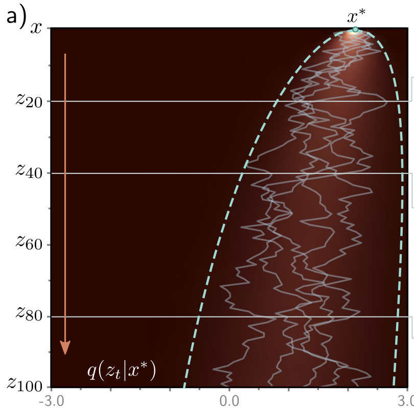
For any starting data point \(x\), variable \(z_t\) is normally distributed with a known mean and variance. If we do not care about the history of the evolution through the intermediate variables, it is easy to generate samples from \(q(z_t|x)\).
The marginal distributions
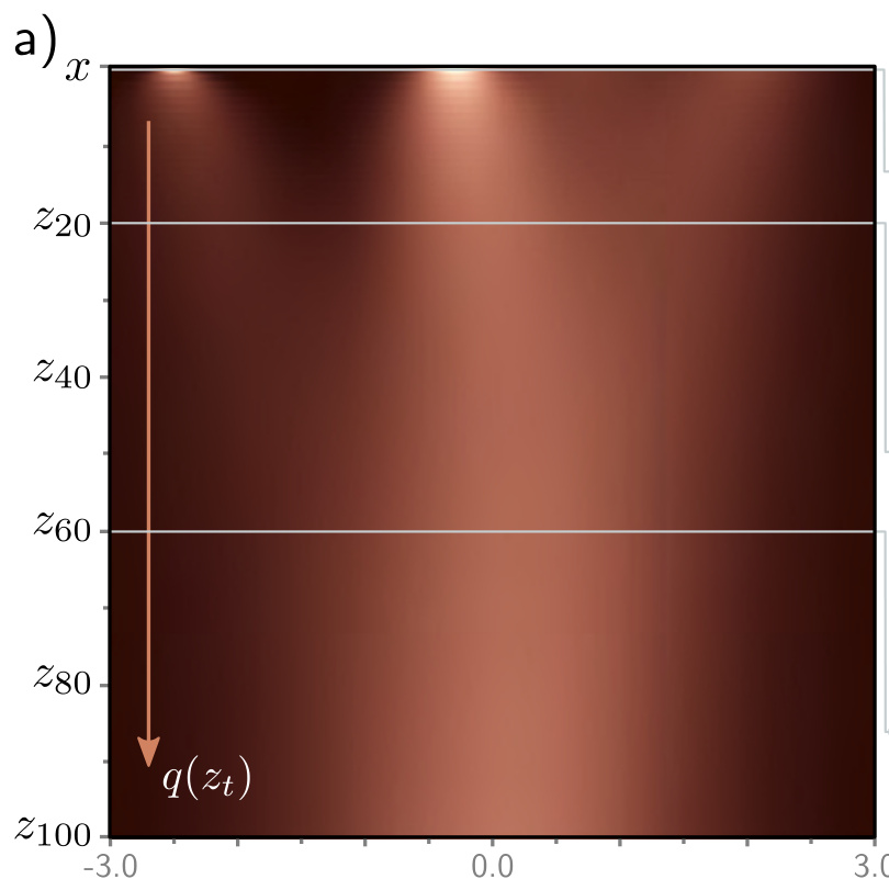
The marginal distribution \(q(z_t)\) is the probability of observing a value of \(z_t\) given the distribution of possible starting points \(x\) and the possible diffusion paths for each. Because the kernel skips the intervening variables, it can be written compactly:
\[ q(z_t) = \int q(z_t|x)\,Pr(x)\,dx . \]
If we repeatedly sample from the data distribution \(Pr(x)\) and superimpose the diffusion kernel on each sample, the result is the marginal distribution. But note the limitation, because we will trip over it in the next section: the marginal distribution cannot be written in closed form, because we do not know the original data distribution \(Pr(x)\).
Key ideas
- Composing Gaussian steps yields another Gaussian, so the whole chain collapses to \(q(z_t|x) = \text{Norm}[\sqrt{\alpha_t}x, (1-\alpha_t)I]\).
- Training can therefore pick a random timestep per example and reach it in one operation.
- \(\alpha_t\) is a running product of \((1-\beta_s)\); as it approaches zero the data term vanishes and the kernel tends to a standard normal.
- The marginal \(q(z_t)\) is a mixture over the data and has no closed form.
Learning outcomes
- diffusion-kernel Use the closed-form diffusion kernel to jump to any noise level in one step.
Concepts
- diffusion-kernel derives \(q(z_t|x) = \text{Norm}[\sqrt{\alpha_t}x, (1-\alpha_t)I]\) by repeatedly substituting the forward step equations, and uses it to define the marginals
- noise-schedule defines \(\alpha_t = \prod_{s=1}^{t}(1-\beta_s)\) directly from the noise schedule
The reverse process and the tractable conditional
We now turn the chain around. Three distributions are in play, and keeping them apart is the whole of this section.
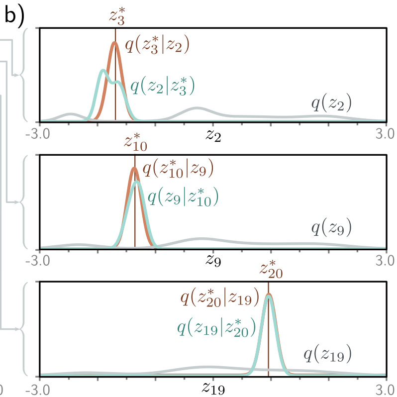
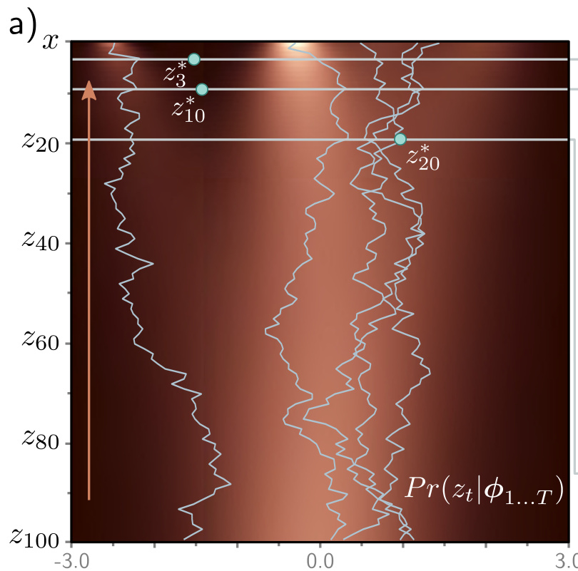
The intractable one: \(q(z_{t-1}|z_t)\)
We defined \(q(z_t|z_{t-1})\) as the mixing process. To reverse it we apply Bayes’ rule:
\[ q(z_{t-1}|z_t) = \frac{q(z_t|z_{t-1})\,q(z_{t-1})}{q(z_t)} . \]
This is intractable, since we cannot compute the marginal distribution \(q(z_{t-1})\). This is precisely the obstacle the variational autoencoder hit with its own posterior.
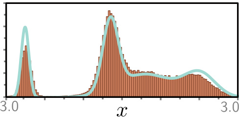
For the simple one-dimensional example it is possible to evaluate \(q(z_{t-1}|z_t)\) numerically. In general its form is complex, but in many cases it is well approximated by a normal distribution. That observation is what licenses the model we are about to write down.
The tractable one: \(q(z_{t-1}|z_t, x)\)
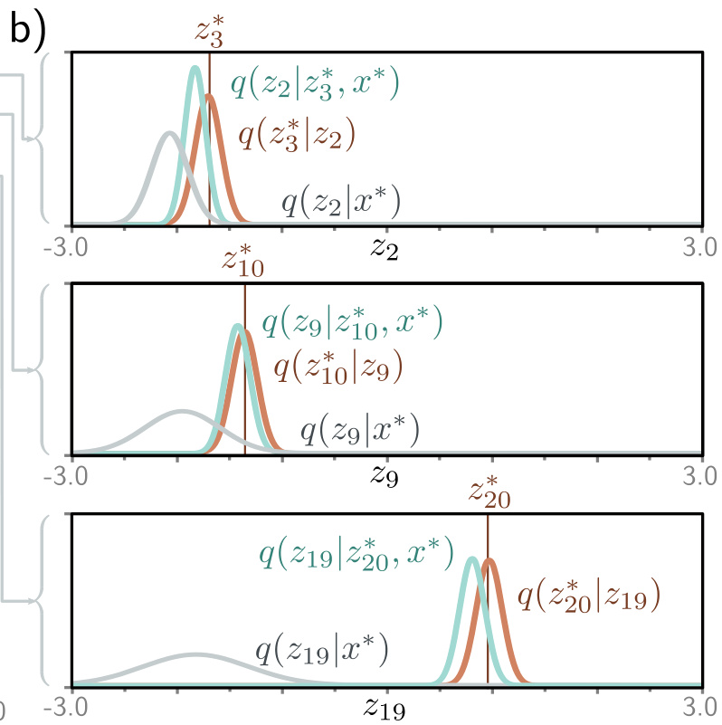
We could not find \(q(z_{t-1}|z_t)\) because we do not know \(q(z_{t-1})\). But if we know the starting variable \(x\), then we do know the distribution \(q(z_{t-1}|x)\) at the time before — that is just the diffusion kernel, and it is normally distributed.
So we start again from Bayes’ rule and keep \(x\) in the conditioning:
\[ q(z_{t-1}|z_t, x) = \frac{q(z_t|z_{t-1},x)\,q(z_{t-1}|x)}{q(z_t|x)} \;\propto\; q(z_t|z_{t-1})\,q(z_{t-1}|x), \]
where \(q(z_t|z_{t-1},x) = q(z_t|z_{t-1})\) because the diffusion process is Markov and all information about \(z_t\) is captured by \(z_{t-1}\). Applying the Gaussian change-of-variables identity to rewrite the first factor in terms of \(z_{t-1}\), then the Gaussian product identity to combine the two, gives a single normal distribution:
\[ q(z_{t-1}|z_t, x) = \text{Norm}_{z_{t-1}}\!\left[\frac{(1-\alpha_{t-1})\sqrt{1-\beta_t}}{1-\alpha_t}z_t + \frac{\sqrt{\alpha_{t-1}}\,\beta_t}{1-\alpha_t}x,\; \frac{\beta_t(1-\alpha_{t-1})}{1-\alpha_t}I\right]. \]
The constants of proportionality must cancel, since the final result is already a correctly normalized probability distribution. This is the distribution over \(z_{t-1}\) when we know the current latent variable \(z_t\) and the training data example \(x\) — and we do know \(x\) when training. It will be the target.
The learned one: the decoder
The true reverse distributions \(q(z_{t-1}|z_t)\) are complex multi-modal distributions that depend on \(Pr(x)\). The reverse (decoder) process approximates them as normal distributions:
\[ \begin{aligned} Pr(z_T) &= \text{Norm}_{z_T}[0, I] \\ Pr(z_{t-1}|z_t, \phi_t) &= \text{Norm}_{z_{t-1}}\!\left[f_t[z_t,\phi_t],\; \sigma_t^2 I\right] \\ Pr(x|z_1, \phi_1) &= \text{Norm}_{x}\!\left[f_1[z_1,\phi_1],\; \sigma_1^2 I\right], \end{aligned} \]
where \(f_t[z_t,\phi_t]\) is a neural network computing the mean of the estimated mapping from \(z_t\) back to \(z_{t-1}\). The variances \(\{\sigma_t^2\}\) are predetermined. If the hyperparameters \(\beta_t\) are close to zero and \(T\) is large, this normal approximation will be reasonable.
We generate new examples using ancestral sampling: draw \(z_T\) from \(Pr(z_T)\), sample \(z_{T-1}\) from \(Pr(z_{T-1}|z_T,\phi_T)\), then \(z_{T-2}\) from \(Pr(z_{T-2}|z_{T-1},\phi_{T-1})\), and so on until we finally generate \(x\) from \(Pr(x|z_1,\phi_1)\).
Learning outcomes
- reverse-process Define the learned reverse process and relate it to the tractable conditional \(q(z_{t-1}|z_t, x)\).
Concepts
- diffusion-kernel applies Bayes’ rule using the diffusion kernel \(q(z_{t-1}|x)\) to obtain the closed-form Gaussian \(q(z_{t-1}|z_t, x)\)
- reverse-process defines the Gaussian transition densities \(Pr(z_{t-1}|z_t,\phi_t)\) and the ancestral sampling algorithm
The diffusion ELBO
The joint distribution of the observed variable and the latents is
\[ Pr(x, z_{1\dots T}|\phi_{1\dots T}) = Pr(x|z_1,\phi_1)\prod_{t=2}^{T} Pr(z_{t-1}|z_t,\phi_t)\cdot Pr(z_T), \]
and the likelihood of the data is found by marginalizing over \(z_{1\dots T}\). We would like to maximise \(\sum_i \log Pr(x_i|\phi_{1\dots T})\), but cannot, because that marginalization is intractable. So we use Jensen’s inequality to define a lower bound and optimize with respect to it, exactly as we did for the VAE.
The bound
Multiply and divide the log-likelihood by the encoder distribution and apply Jensen’s inequality:
\[ \log\left[Pr(x|\phi_{1\dots T})\right] = \log\left[\int q(z_{1\dots T}|x)\frac{Pr(x,z_{1\dots T}|\phi_{1\dots T})}{q(z_{1\dots T}|x)}dz_{1\dots T}\right] \ge \int q(z_{1\dots T}|x)\log\left[\frac{Pr(x,z_{1\dots T}|\phi_{1\dots T})}{q(z_{1\dots T}|x)}\right]dz_{1\dots T}. \]
The right-hand side is the evidence lower bound (ELBO) for diffusion.
In the VAE, the encoder approximates the posterior to make the bound tight and the decoder maximizes it. In diffusion models the decoder must do all the work, since the encoder has no parameters. It tightens the bound by both changing its parameters so that the static encoder does approximate the posterior \(Pr(z_{1\dots T}|x,\phi_{1\dots T})\), and optimizing its own parameters with respect to that bound.
Simplifying it
Substituting the two products into the log and separating terms gives
\[ \log\left[\frac{Pr(x,z_{1\dots T}|\phi)}{q(z_{1\dots T}|x)}\right] = \log\left[\frac{Pr(x|z_1,\phi_1)}{q(z_1|x)}\right] + \log\left[\frac{\prod_{t=2}^{T}Pr(z_{t-1}|z_t,\phi_t)}{\prod_{t=2}^{T}q(z_t|z_{t-1})}\right] + \log\left[Pr(z_T)\right]. \]
The pivotal move is to expand the denominator of the middle term using the Markov property and Bayes’ rule:
\[ q(z_t|z_{t-1}) = q(z_t|z_{t-1},x) = \frac{q(z_{t-1}|z_t,x)\,q(z_t|x)}{q(z_{t-1}|x)} . \]
The first equality holds because all information about \(z_t\) is encompassed in \(z_{t-1}\), so the extra conditioning on \(x\) is irrelevant. Substituting this in, the ratios \(q(z_{t-1}|x)/q(z_t|x)\) telescope: all but two cancel, leaving only \(q(z_1|x)\) and \(q(z_T|x)\). The surviving \(\log[Pr(z_T)/q(z_T|x)]\) is approximately \(\log[1] = 0\), since the result of the forward process \(q(z_T|x)\) is a standard normal distribution and so is equal to the prior \(Pr(z_T)\). What remains is
\[ \text{ELBO}[\phi_{1\dots T}] \approx \mathbb{E}_{q(z_1|x)}\!\left[\log Pr(x|z_1,\phi_1)\right] - \sum_{t=2}^{T}\mathbb{E}_{q(z_t|x)}\!\left[D_{KL}\!\left[q(z_{t-1}|z_t,x)\,\big\|\,Pr(z_{t-1}|z_t,\phi_t)\right]\right]. \]
Reading the terms
The first term is the reconstruction term, equivalent to the VAE’s. The ELBO is larger if the model prediction matches the observed data. We approximate the expectation with a Monte Carlo sample from \(q(z_1|x)\).
It is a log normal, so it will later become a least-squares term like the rest.
Each remaining term measures the distance between the decoder step \(Pr(z_{t-1}|z_t,\phi_t)\) and the tractable conditional \(q(z_{t-1}|z_t,x)\). Both are spherical Gaussians we know in closed form.
Many terms in the KL expression do not depend on \(\phi\), so it simplifies to the squared difference between the means plus a constant \(C\): \[D_{KL}\left[\cdot\,\|\,\cdot\right] = \frac{1}{2\sigma_t^2}\left\|\frac{(1-\alpha_{t-1})\sqrt{1-\beta_t}}{1-\alpha_t}z_t + \frac{\sqrt{\alpha_{t-1}}\beta_t}{1-\alpha_t}x - f_t[z_t,\phi_t]\right\|^2 + C.\]
Recasting maximisation as minimisation and approximating expectations with samples gives the loss function
\[ L[\phi_{1\dots T}] = \sum_{i=1}^{I}\left(-\log\text{Norm}_{x_i}\!\left[f_1[z_{i1},\phi_1],\sigma_1^2 I\right] + \sum_{t=2}^{T}\frac{1}{2\sigma_t^2}\left\|\underbrace{\frac{1-\alpha_{t-1}}{1-\alpha_t}\sqrt{1-\beta_t}\,z_{it} + \frac{\sqrt{\alpha_{t-1}}\beta_t}{1-\alpha_t}x_i}_{\text{target: mean of } q(z_{t-1}|z_t,x)} - \underbrace{f_t[z_{it},\phi_t]}_{\text{predicted } z_{t-1}}\right\|^2\right). \]
An intimidating variational bound has become a per-step regression problem. The network at step \(t\) must predict the most likely value of \(z_{t-1}\) given the ground-truth denoised data \(x\).
Learning outcomes
- diffusion-elbo Derive the diffusion ELBO and simplify it into a sum of per-timestep KL terms.
Concepts
- diffusion-elbo derives the bound from Jensen’s inequality for a parameter-free encoder, expands the joint ratio into a sum of KL divergences, and reduces each to a squared difference of means
The noise-prediction objective
The loss above can be used, but diffusion models have been found to work better with a different parameterization. The loss function is modified so that the model aims to predict the noise that was mixed with the original data example to create the current variable. Two substitutions get us there: one on the target, one on the network.
Reparameterizing the target
The diffusion kernel says \(z_t = \sqrt{\alpha_t}\cdot x + \sqrt{1-\alpha_t}\cdot\epsilon\). It follows that the data term \(x\) can be expressed as the diffused image minus the noise that was added to it:
\[ x = \frac{1}{\sqrt{\alpha_t}}\cdot z_t - \frac{\sqrt{1-\alpha_t}}{\sqrt{\alpha_t}}\cdot\epsilon . \]
Substituting this into the target and simplifying — using \(\sqrt{\alpha_t}/\sqrt{\alpha_{t-1}} = \sqrt{1-\beta_t}\) along the way — collapses the whole expression to two terms:
\[ \frac{1-\alpha_{t-1}}{1-\alpha_t}\sqrt{1-\beta_t}\,z_t + \frac{\sqrt{\alpha_{t-1}}\beta_t}{1-\alpha_t}x \;=\; \frac{1}{\sqrt{1-\beta_t}}z_t - \frac{\beta_t}{\sqrt{1-\alpha_t}\sqrt{1-\beta_t}}\epsilon . \]
The target no longer mentions \(x\) at all. It mentions \(z_t\), which the network sees, and \(\epsilon\), which it does not — but which it could plausibly learn to predict.
Reparameterizing the network
Now replace the model \(\hat z_{t-1} = f_t[z_t,\phi_t]\) with a new model \(\hat\epsilon = g_t[z_t,\phi_t]\), which predicts the noise \(\epsilon\) that was mixed with \(x\) to create \(z_t\):
\[ f_t[z_t,\phi_t] = \frac{1}{\sqrt{1-\beta_t}}z_t - \frac{\beta_t}{\sqrt{1-\alpha_t}\sqrt{1-\beta_t}}g_t[z_t,\phi_t] . \]
The \(z_t\) terms in target and prediction are now identical and cancel. What is left is a scaled squared difference between the true noise and the predicted noise:
\[ L[\phi_{1\dots T}] = \sum_{i=1}^{I}\left(-\log\text{Norm}_{x_i}\!\left[f_1[z_{i1},\phi_1],\sigma_1^2 I\right] + \sum_{t=2}^{T}\frac{\beta_t^2}{(1-\alpha_t)(1-\beta_t)2\sigma_t^2}\left\|g_t[z_{it},\phi_t] - \epsilon_{it}\right\|^2\right). \]
The log normal can itself be written as a least-squares loss plus a constant, and substituting the definitions of \(x\) and \(f_1\) shows that the reconstruction term takes exactly the same form as the others with \(t=1\). Adding it back and discarding the additive constants:
\[ L[\phi_{1\dots T}] = \sum_{i=1}^{I}\sum_{t=1}^{T}\frac{\beta_t^2}{(1-\alpha_t)(1-\beta_t)2\sigma_t^2}\left\|g_t[z_{it},\phi_t] - \epsilon_{it}\right\|^2 . \]
In practice, the scaling factors — which might be different at each time step — are ignored, giving an even simpler formulation:
\[ L[\phi_{1\dots T}] = \sum_{i=1}^{I}\sum_{t=1}^{T}\left\|g_t[z_{it},\phi_t] - \epsilon_{it}\right\|^2 = \sum_{i=1}^{I}\sum_{t=1}^{T}\left\|g_t\!\left[\sqrt{\alpha_t}\cdot x_i + \sqrt{1-\alpha_t}\cdot\epsilon_{it},\, \phi_t\right] - \epsilon_{it}\right\|^2, \]
where the second line rewrites \(z_{it}\) using the diffusion kernel.
Nothing in the final line looks probabilistic. A variational bound over a chain of \(T\) latent variables has become: corrupt an example to a random noise level, ask the network what noise you added, and penalise the squared error. The dropped per-timestep weights are the one place where the derivation and the practice part company, and the departure is empirical — equal weighting was found to improve sample quality.
Learning outcomes
- noise-prediction-loss Reparameterize target and network to obtain the simple noise-prediction loss.
Concepts
- noise-prediction-reparameterization substitutes \(x\) expressed via \(\epsilon\) into the target mean, then defines the noise-predicting network \(g_t\), yielding the standard unweighted mean-squared-error loss
Training and sampling algorithms
The simplified loss leads to straightforward algorithms for both training and sampling. State them precisely, because the asymmetry between them shapes everything that follows.
Training
Algorithm 18.1: Diffusion model training
  Input:  Training data x
  Output: Model parameters phi_t
  repeat
     for i in B do                          // For every training example index in batch
         t ~ Uniform[1, ... T]              // Sample random timestep
         eps ~ Norm[0, I]                   // Sample noise
         l_i = || g_t[ sqrt(alpha_t) x_i + sqrt(1-alpha_t) eps, phi_t ] - eps ||^2
     Accumulate losses for batch and take gradient step
  until converged
Two advantages are worth naming. The procedure is simple to implement. And it naturally augments the dataset: we can reuse every original data point \(x_i\) as many times as we want at each time step with different noise instantiations \(\epsilon\).
Sampling
Algorithm 18.2: Sampling
  Input:  Model, g_t[., phi_t]
  Output: Sample, x
  z_T ~ Norm_z[0, I]                        // Sample last latent variable
  for t = T ... 2 do
      zhat_{t-1} = z_t/sqrt(1-beta_t) - beta_t/(sqrt(1-alpha_t) sqrt(1-beta_t)) g_t[z_t, phi_t]
      eps ~ Norm_eps[0, I]                  // Draw new noise vector
      z_{t-1} = zhat_{t-1} + sigma_t eps    // Add noise to previous latent variable
  x = z_1/sqrt(1-beta_1) - beta_1/(sqrt(1-alpha_1) sqrt(1-beta_1)) g_1[z_1, phi_1]
Note the last line. The loop runs down to \(t=2\); the final step from \(z_1\) to \(x\) generates the sample without adding noise.
Training is one network evaluation per gradient step, and every example can be sent to any timestep in a single operation. Sampling requires serial processing of many neural networks \(g_t[z_t,\phi_t]\) and is hence time-consuming. The evaluations cannot be parallelised, because each depends on the output of the last. This is the single largest practical objection to diffusion models, and we address it two sections from now.
Learning outcomes
- training-and-sampling-loops Write the training loop and the ancestral sampling loop for a diffusion model.
- noise-prediction-loss Reparameterize target and network to obtain the simple noise-prediction loss.
Implementing diffusion for images
Diffusion models have been very successful in modeling image data. Here we need to construct models that can take a noisy image and predict the noise that was added at each step. The output has the same shape as the input, because it is itself a noise image.
The obvious architectural choice for this image-to-image mapping is the U-Net. Its downsampling path supplies global context, and its skip connections carry fine spatial detail across to the decoder.
Both are needed. Early steps of the reverse chain settle layout; late steps settle texture.
One network, not \(T\) of them. There may be a very large number of diffusion steps, and training and storing multiple U-Nets is inefficient. The solution is to train a single U-Net that also takes a predetermined vector representing the time step as input.
In practice, this vector is resized to match the number of channels at each stage of the U-Net and used to offset and/or scale the representation at each spatial position.
Time conditioning is sinusoidal. A sinusoidal time embedding is passed through a shallow neural network and the result is added to the channels at every spatial position at every stage of the U-Net.
The same weights therefore behave differently at different noise levels, which is what makes sharing them across \(t\) workable.
Attention is periodic and global. Connections between adjacent representations consist of residual blocks, with periodic global self-attention in which every spatial position interacts with every other spatial position.
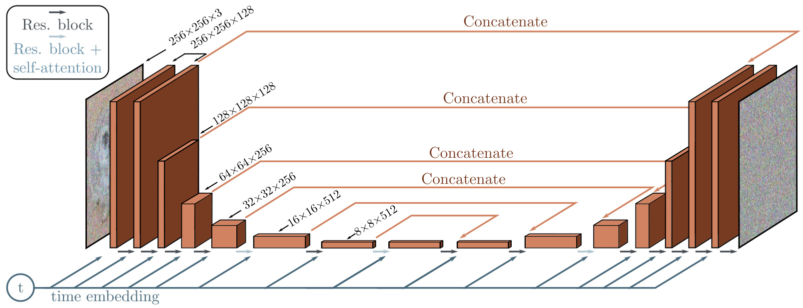
The number of time steps is not a free choice. A large number of steps is needed because the conditional probabilities \(q(z_{t-1}|z_t)\) become closer to normal when the hyperparameters \(\beta_t\) are close to zero — matching the form of the decoder distributions \(Pr(z_{t-1}|z_t,\phi_t)\) we committed to. However, this makes sampling slow. We might have to run the U-Net model through \(T = 1000\) steps to generate good images.
Stable diffusion (Rombach et al., 2022) projects the original data to a smaller latent space using a conventional autoencoder and runs the diffusion process there. This reduces the dimensionality the diffusion process must handle, and allows other data types to be described by diffusion models.
Learning outcomes
- image-implementation Explain how a diffusion model is implemented for images with a time-conditioned U-Net.
Concepts
- noise-prediction-reparameterization presents the concrete training and sampling algorithms built around noise prediction
Faster sampling
The route to faster sampling begins with an observation about the loss function. The loss requires the diffusion kernel to have the form \(q(z_t|x) = \text{Norm}[\sqrt{\alpha_t}x, (1-\alpha_t)I]\). The same loss function will be valid for any forward process with this relation, and there is a family of such compatible processes.
These are all optimized by the same loss function but have different rules for the forward process, and different corresponding rules for how to use the estimated noise \(g[z_t,\phi_t]\) to predict \(z_{t-1}\) from \(z_t\) in the reverse process. A model already trained can therefore be sampled under a different member of the family without retraining.
Two members matter in practice.
Denoising diffusion implicit models (DDIM). These are no longer stochastic after the first step from \(x\) to \(z_1\). The reverse trajectory becomes deterministic.
Song et al. (2021a) showed the family is largely non-Markovian: the diffusion step does not depend only on the results of the previous step. DDIM is amenable to taking larger steps without inducing large errors.
Accelerated sampling models, where the forward process is defined only on a sub-sequence of time steps. This allows a reverse process that skips time steps and hence makes sampling much more efficient.
Good samples can be created with 50 time steps when the forward process is no longer stochastic. This is much faster than before but still slower than most other generative models.
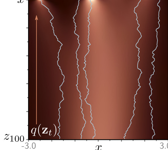
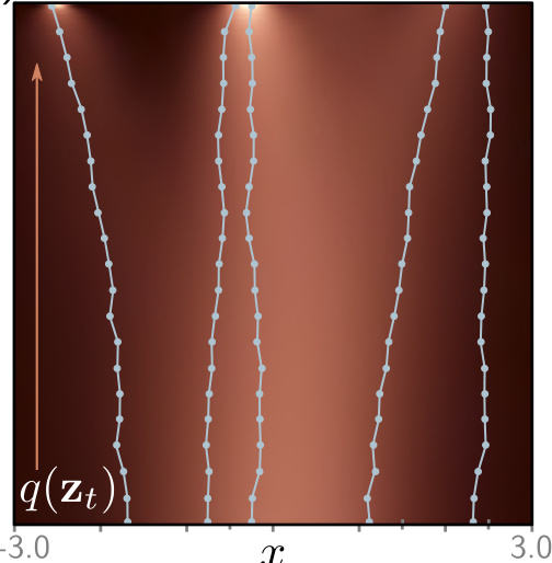
The deterministic view generalises. DDIM effectively converts the model into an ordinary differential equation in which the trajectories have low curvature, allowing efficient numerical methods for solving ODEs to be applied. Song et al. (2021c) propose converting the underlying stochastic differential equations into a probability flow ODE which has the same marginal distributions as the original process. Karras et al. (2022) identified the best-performing time discretization for sampling and evaluated different sampler schedules.
There are two further lines of attack recorded in the chapter’s notes. Salimans & Ho (2022) distilled adjacent steps of the denoising process into a single step. And one can attack the root cause instead: sampling is slow because many small steps are required to keep \(q(z_{t-1}|z_t)\) close to Gaussian. If we use a model that describes a more complex distribution at each denoising step, we can use fewer diffusion steps in the first place — conditional GANs and conditional energy-based models have both been tried in that role.
Learning outcomes
- faster-sampling Accelerate sampling with deterministic and step-skipping formulations.
Concepts
- ddim explains how denoising diffusion implicit models use a deterministic, non-Markovian forward process to skip inference steps
Conditioning and scaling up
If the data has associated labels \(c\), these can be exploited to control the generation. The intuition is plain: it is easier to denoise an image if you have some information about what that image contains.
Classifier guidance
Classifier guidance modifies the denoising update from \(z_t\) to \(z_{t-1}\) to take account of class information \(c\). In practice this means adding an extra term into the final update step of Algorithm 18.2:
\[ z_{t-1} = \hat z_{t-1} + \sigma_t^2\left(\frac{\partial \log Pr(c|z_t)}{\partial z_t}\right) + \sigma_t\epsilon . \]
The new term depends on the gradient of a classifier \(Pr(c|z_t)\) that is based on the latent variable \(z_t\). This maps features from the downsampling half of the U-Net to the class \(c\). Like the U-Net, it is usually shared across all time steps and takes time as an input. The update from \(z_t\) to \(z_{t-1}\) now makes the class \(c\) more likely. The cost is that a separate classifier, one that works on noisy inputs at every noise level, must be trained.
Classifier-free guidance
Classifier-free guidance avoids learning a separate classifier and instead incorporates class information into the main model \(g_t[z_t,\phi_t,c]\). In practice this usually takes the form of adding an embedding based on \(c\) to the layers of the U-Net, in a similar way to how the time step is added.
The model is jointly trained on conditional and unconditional objectives by randomly dropping the class information during training. Hence it can generate unconditional or conditional data examples at test time, or any weighted combination of the two. This brings a surprising advantage: if the conditioning information is over-weighted, the model tends to produce very high quality but slightly stereotypical examples. This is somewhat analogous to the use of truncation in GANs.
This is deliberately an overview. The mechanics of guidance — why the weighted extrapolation is the right thing to compute, and what the guidance weight trades away — are taken up properly in the later units of this module on classifier-guided and classifier-free diffusion.
Scaling to high resolution
The highest quality results come from a combination of extensions.
- Learn the reverse variances. It helps to estimate the variances \(\sigma_t^2\) of the reverse process as well as the mean. This particularly improves results when sampling with fewer steps.
- Vary the noise schedule. It is possible to modify the forward process so that \(\beta_t\) varies at each step, and this can also improve results.
- Use a cascade. To generate high-resolution images, a cascade of diffusion models is used. The first creates a low-resolution image, possibly guided by class information. Subsequent models generate progressively higher-resolution images, conditioning on the lower-resolution image by resizing it and appending it to the layers of the constituent U-Net, as well as on any other class information.
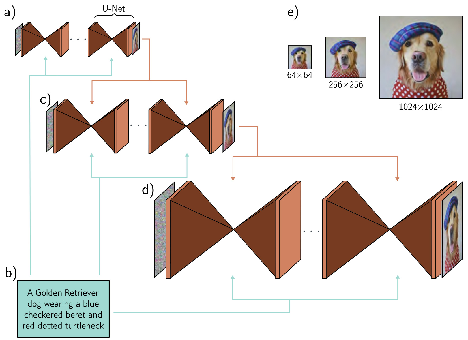
Text conditioning enters the same way. A model trained to condition on text captions encoded by a language model inserts those encodings into the network exactly as the time step is inserted. Since the diffusion model is stochastic by nature, it is possible to generate multiple images conditioned on the same caption.
To stop artifacts in the lower-resolution image propagating upward, Ho et al. (2022a) introduced noise conditioning augmentation: the conditioning image is degraded by adding noise at each training step, reducing reliance on its exact details.
Learning outcomes
- conditioning-and-scaling Condition generation on class or text and scale to high resolution with cascades.
Concepts
- classifier-guidance describes modifying the reverse step by adding the gradient \(\nabla_{z_t}\log Pr(c|z_t)\)
- classifier-free-guidance explains conditioning directly inside the U-Net and randomly dropping class labels during training
- cascaded-diffusion explains how multiple diffusion models sequentially upscale images from low to high resolution
Consolidation, and where the text comes from
Diffusion models map the data examples through a series of latent variables by repeatedly blending the current representation with random noise. After sufficient steps, the representation becomes indistinguishable from white noise. Since these steps are small, the reverse denoising process at each step can be approximated with a normal distribution and predicted by a deep learning model. The loss function is based on the evidence lower bound and ultimately results in a simple least-squares formulation.
What you can now do:
- Write the forward chain \(z_t = \sqrt{1-\beta_t}z_{t-1} + \sqrt{\beta_t}\epsilon_t\) and say what the schedule controls.
- Use the diffusion kernel \(q(z_t|x) = \text{Norm}[\sqrt{\alpha_t}x,(1-\alpha_t)I]\) to reach any noise level in one operation.
- Distinguish the intractable \(q(z_{t-1}|z_t)\) from the closed-form \(q(z_{t-1}|z_t,x)\), and say why the latter supervises the decoder.
- Derive the ELBO for the chain, reduce it to per-step Gaussian KL terms, and reparameterize it into \(\|g_t[z_t,\phi_t]-\epsilon\|^2\).
- Write both loops, implement \(g_t\) as a time-conditioned U-Net, accelerate sampling with DDIM or an ODE solver, and condition on a class or a prompt.
Two costs are worth carrying forward as honestly as the strengths. Diffusion models are slow, and the latent space has no semantic interpretation. In their basic form they compute only a lower bound on the likelihood of a data point — though Kingma et al. (2021) show that this bound improves on the exact log-likelihoods obtained from normalizing flows and autoregressive models on test data.
Where this goes next — 2021 CLIP. Conditioning on a text prompt in this unit assumed a sentence embedding without saying where it comes from. The chapter’s own notes point at the answer: GLIDE and DALL·E 2 are both conditioned on embeddings from the CLIP model of Radford et al. (2021), which generates joint embeddings for text and image data. The next unit reads that paper. Because the two encoders are trained into a shared space, a text embedding can score an image — and that is what makes text-driven guidance of a diffusion model possible at all. After CLIP, the module returns to guided diffusion and assembles text-to-image generation from these two halves.
Learning outcomes
- forward-process Describe the fixed forward noising process and the role of the variance schedule.
- diffusion-kernel Use the closed-form diffusion kernel to jump to any noise level in one step.
- reverse-process Define the learned reverse process and relate it to the tractable conditional \(q(z_{t-1}|z_t, x)\).
- diffusion-elbo Derive the diffusion ELBO and simplify it into a sum of per-timestep KL terms.
- noise-prediction-loss Reparameterize target and network to obtain the simple noise-prediction loss.
- training-and-sampling-loops Write the training loop and the ancestral sampling loop for a diffusion model.
- image-implementation Explain how a diffusion model is implemented for images with a time-conditioned U-Net.
- faster-sampling Accelerate sampling with deterministic and step-skipping formulations.
- conditioning-and-scaling Condition generation on class or text and scale to high resolution with cascades.
Concepts
- diffusion-model summarizes the end-to-end forward noise addition and reverse neural denoising process
- diffusion-elbo recaps how the ELBO formulation reduces to simple least-squares regression
- ddim references the introduction and properties of DDIM by Song et al.
- classifier-guidance cites Dhariwal & Nichol (2021) regarding classifier guidance
- classifier-free-guidance cites Ho & Salimans (2022) for classifier-free guidance
- cascaded-diffusion cites Ho et al. (2022a) for cascaded diffusion pipelines
References
- Understanding Deep Learning, Simon Prince, 2026 — Link — Page 363-387