Lecture notes — CLIP Guided Image Diffusion
ver. 1.0.0, clip_guided_image_diffusion
ver. 1.0.0 · 2026-08-22 10:25:20
Where we are
You arrive at this unit with two pieces already in hand. From the diffusion unit you have a reverse chain in which each step is a Gaussian whose mean is computed from a noise-predicting U-Net. From 2021 Clip you have an image encoder \(f\) and a text encoder \(g\) that share one embedding space, so that the dot product \(f(x)\cdot g(c)\) scores how well an image \(x\) matches a caption \(c\).
This unit joins them. The joining device is a gradient: if some differentiable function scores how well a partially denoised image matches a target, its gradient can be added to the reverse step, nudging the chain toward images that score well. We study two papers that build this out — Dhariwal and Nichol’s Diffusion Models Beat GANs on Image Synthesis, which introduces the mechanism and the architecture that made it worth having, and Nichol et al.’s GLIDE, which replaces the classifier with CLIP and the class label with free-form text.
What you will be able to do
metrics-and-architecture— Evaluate diffusion samples with the standard metrics and describe the U-Net changes that improved them.classifier-guidance-derivation— Derive the classifier-guided reverse step and its DDIM counterpart.gradient-scale-tradeoff— Use the gradient scale to trade sample diversity for fidelity.classifier-guided-results— Report what classifier-guided diffusion achieved against GANs, and at what cost.text-conditional-diffusion— Describe how GLIDE conditions a diffusion U-Net on free-form text.clip-guidance— Guide a diffusion model with a CLIP score, using a noise-aware CLIP.comparing-guidance-strategies— Compare CLIP guidance against classifier-free guidance and explain why the CLIP score misleads.inpainting-and-editing— Fine-tune a text-conditional diffusion model for text-guided inpainting and editing.safety-and-limitations— Assess the safety case for releasing a text-to-image model, and what these models still cannot do.
What we will cover
The two papers introduce nine concepts between them.
- Classifier guidance — steering diffusion sampling with gradients from a classifier trained on noisy images.
- Classifier gradient scale — a scaling hyperparameter on those gradients that trades diversity for fidelity.
- Ablated Diffusion Model (ADM) — the U-Net refined by ablation: multi-resolution attention, 64 channels per head, BigGAN residual blocks.
- Adaptive group normalization (AdaGN) — a layer that conditions residual blocks on timestep and class embeddings by scale and shift.
- Two-stage upsampling stack (ADM-U) — a low-resolution model followed by a separate conditional super-resolution diffusion model.
- GLIDE — a text-conditional diffusion base model plus upsampler for photorealistic generation and editing.
- Noised CLIP guidance — guidance from a CLIP image encoder trained on noised images.
- Classifier-free guidance — guidance from one model’s own conditional and unconditional predictions.
- Text-conditional inpainting — fine-tuning with mask and context channels for language-driven local edits.
Joining CLIP to diffusion
Two ingredients meet in this unit, and it is worth being precise about what each one supplies.
The diffusion model supplies a generator that is steerable by a gradient. Its reverse step is a Gaussian \(\mathcal{N}(\mu, \Sigma)\), and a Gaussian’s mean can be displaced. Nothing in the sampler forbids displacing it by a quantity computed from another network. The question is which displacement corresponds to conditioning, and that question has an answer we will derive.
CLIP supplies the score. The quantity \(f(x)\cdot g(c)\) is differentiable in \(x\), and \(c\) may be any caption at all. That removes the restriction that has followed classifier guidance from the start: a classifier can only say which of a fixed set of labels an image belongs to.
Two papers carry the story.
Classifier-guided diffusion. Dhariwal and Nichol derive guidance from the reverse transition, catalogue the U-Net changes that made diffusion competitive before any guidance was applied, and identify the gradient scale as the single knob that trades fidelity against diversity. This is where diffusion models overtook GANs.
They report an FID of 2.97 on ImageNet \(128\times128\), 4.59 on \(256\times256\) and 7.72 on \(512\times512\), matching BigGAN-deep with as few as 25 forward passes per sample.
GLIDE. Nichol et al. take the same architecture, condition it on free-form text at 3.5 billion parameters, and put CLIP guidance head to head against classifier-free guidance. The comparison does not go the way the CLIP score predicts.
GLIDE stands for Guided Language to Image Diffusion for Generation and Editing. The smaller model trained on filtered data is called GLIDE (filtered).
Read the unit with one question in view: what does a piece of guidance cost? Every method we study buys fidelity with something — coverage, a second network, a training run, or the trustworthiness of the metric you are measuring with.
Learning outcomes
- classifier-guidance-derivation Derive the classifier-guided reverse step and its DDIM counterpart.
- clip-guidance Guide a diffusion model with a CLIP score, using a noise-aware CLIP.
- text-conditional-diffusion Describe how GLIDE conditions a diffusion U-Net on free-form text.
Metrics and architecture improvements
Before anything is guided, two unglamorous things must be settled: how sample quality is measured, and whether the backbone is any good. Much of the gain in Dhariwal and Nichol’s paper comes from the second, and could not have been detected without the first.
The measuring stick
The paper evaluates with four families of metric, and warns that none is a perfect proxy.
Inception Score (IS) measures how well a model captures the full ImageNet class distribution while still producing individual samples that are convincing examples of a single class.
Its drawback is that it does not reward covering the whole distribution or capturing diversity within a class. A model that memorises a small subset of the dataset still scores highly.
Fréchet Inception Distance (FID) is a symmetric measure of the distance between two image distributions in the Inception-V3 latent space. It is the paper’s default metric, because it captures both diversity and fidelity.
sFID is a version of FID computed on spatial features rather than pooled features, and so rewards coherent high-level structure.
Improved Precision and Recall separate the two things FID mixes: precision is the fraction of model samples falling into the data manifold, recall the fraction of data samples falling into the sample manifold.
The paper uses Precision or IS to measure fidelity and Recall to measure diversity, and uses the entire training set as the reference batch so that comparisons across papers are not distorted by different reference subsets.
Guidance moves fidelity and diversity in opposite directions. A method reported with IS alone will look like an unqualified improvement. Reported with Recall as well, it looks like a trade.
The backbone
The starting point is the DDPM U-Net: residual layers with downsampling convolutions, then residual layers with upsampling convolutions, skip connections between equal resolutions, one global attention layer at \(16\times16\) with a single head, and a projection of the timestep embedding into each residual block. Five changes were ablated on ImageNet \(128\times128\).
- Increasing depth versus width, holding model size roughly constant.
- Increasing the number of attention heads.
- Attention at \(32\times32\), \(16\times16\) and \(8\times8\) rather than only at \(16\times16\).
- BigGAN residual blocks for upsampling and downsampling the activations.
- Rescaling residual connections by \(\frac{1}{\sqrt 2}\).
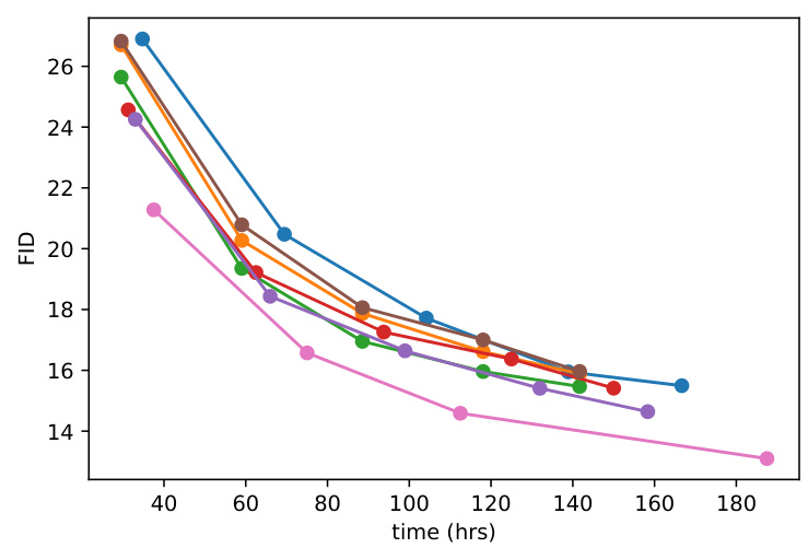
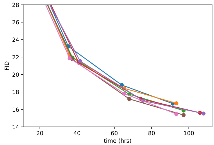
All but the last improved FID, and their effects compounded: the combined model moved FID by \(-3.14\) at 700K iterations and \(-3.00\) at 1200K. Depth helped, but increased training time, so width was preferred over depth. On attention, the paper found that more heads or fewer channels per head improve FID — 32 channels per head gave the largest FID gain — but chose 64 channels per head as the default, because Figure 2 shows 64 is best for wall-clock time and on par with the alternatives in final FID.
Adaptive group normalization
The remaining question is how conditioning information reaches the network at all. Adaptive group normalization (AdaGN) is the answer the paper settles on. It is defined as
\[\mathrm{AdaGN}(h, y) = y_s\,\mathrm{GroupNorm}(h) + y_b\]
where \(h\) is the intermediate activation of the residual block following the first convolution, and \(y = [y_s, y_b]\) is obtained from a linear projection of the timestep and class embedding. It is the analogue for diffusion of adaptive instance norm and FiLM.
Ablated against the Addition + GroupNorm layer of the original DDPM, AdaGN gives FID 13.06 against 15.08. Both models used 128 base channels, 2 residual blocks per resolution, multi-resolution attention with 64 channels per head, BigGAN up- and downsampling, and 700K iterations of training.
The final architecture — variable width with 2 residual blocks per resolution, multiple heads at 64 channels each, attention at 32, 16 and 8, BigGAN residual blocks for resampling, and AdaGN — is the Ablated Diffusion Model (ADM), and is used unchanged for the rest of both papers.
Key ideas
- FID is the default metric; IS and Precision measure fidelity, Recall measures diversity.
- Architecture alone moved FID by about three points before any guidance was applied.
- AdaGN is the channel through which timestep and class information enters every residual block.
- Do not attribute to guidance what belongs to the backbone.
Learning outcomes
- metrics-and-architecture Evaluate diffusion samples with the standard metrics and describe the U-Net changes that improved them.
Concepts
- ablated-diffusion-model AdaGN is evaluated and selected as an essential component of the final ablated diffusion model architecture
- adaptive-group-normalization provides the mathematical definition and ablation results for adaptive group normalization
Deriving classifier guidance
Conditional GANs make heavy use of class labels, through class-conditional normalisation statistics and through discriminator heads explicitly designed to behave like classifiers \(p(y|x)\). ADM already puts class information into its normalisation layers. Here we take a different route: exploit a classifier \(p(y|x)\) to improve a diffusion generator that has already been trained.
The plan is to train a classifier \(p_\phi(y|x_t, t)\) on noisy images \(x_t\), and use its gradients \(\nabla_{x_t}\log p_\phi(y|x_t, t)\) to steer sampling toward a label \(y\). For brevity we write \(p_\phi(y|x_t)\) and \(\epsilon_\theta(x_t)\), remembering that both are conditioned on \(t\).
The conditional reverse noising process
Start with an unconditional reverse process \(p_\theta(x_t|x_{t+1})\). To condition it on a label \(y\), it suffices to sample each transition from
\[p_{\theta,\phi}(x_t|x_{t+1}, y) = Z\,p_\theta(x_t|x_{t+1})\,p_\phi(y|x_t)\]
with \(Z\) a normalising constant. Sampling from this exactly is intractable. But the diffusion model’s own transition is Gaussian,
\[p_\theta(x_t|x_{t+1}) = \mathcal{N}(\mu, \Sigma), \qquad \log p_\theta(x_t|x_{t+1}) = -\tfrac{1}{2}(x_t-\mu)^T\Sigma^{-1}(x_t-\mu) + C\]
and we may assume \(\log p_\phi(y|x_t)\) has low curvature compared with \(\Sigma^{-1}\). That assumption is reasonable in the limit of infinitely many diffusion steps, where \(\|\Sigma\|\to 0\). A first-order Taylor expansion around \(x_t = \mu\) then gives
\[\log p_\phi(y|x_t) \approx \log p_\phi(y|x_t)\big|_{x_t=\mu} + (x_t-\mu)\,g = (x_t-\mu)g + C_1\]
with \(g = \nabla_{x_t}\log p_\phi(y|x_t)\big|_{x_t=\mu}\). Adding this to the Gaussian’s log-density and completing the square,
\[\log\big(p_\theta(x_t|x_{t+1})p_\phi(y|x_t)\big) \approx -\tfrac{1}{2}(x_t-\mu-\Sigma g)^T\Sigma^{-1}(x_t-\mu-\Sigma g) + C_3\]
which is \(\log p(z)\) for \(z \sim \mathcal{N}(\mu + \Sigma g, \Sigma)\), up to a constant we may discard because it corresponds to \(Z\).
The conclusion is worth stating plainly. The conditional transition is the same Gaussian as the unconditional one, with its mean shifted by \(\Sigma g\). The covariance is unchanged. Guidance therefore costs one classifier backward pass per sampling step and nothing else.
Algorithm 1 Classifier guided diffusion sampling, given a diffusion model
(mu_theta(x_t), Sigma_theta(x_t)), classifier p_phi(y|x_t), and gradient scale s.
  Input: class label y, gradient scale s
  x_T <- sample from N(0, I)
  for all t from T to 1 do
    mu, Sigma <- mu_theta(x_t), Sigma_theta(x_t)
    x_{t-1} <- sample from N(mu + s Sigma grad_{x_t} log p_phi(y|x_t), Sigma)
  end for
  return x_0
Conditional sampling for DDIM
The derivation above is valid only for the stochastic sampler. DDIM has no reverse noise to shift, so a different route is needed. It uses the connection between diffusion models and score matching: a noise-prediction model gives a score function
\[\nabla_{x_t}\log p_\theta(x_t) = -\frac{1}{\sqrt{1-\bar\alpha_t}}\,\epsilon_\theta(x_t)\]
Substituting into the score of the joint distribution \(p(x_t)p_\phi(y|x_t)\),
\[\nabla_{x_t}\log\big(p_\theta(x_t)p_\phi(y|x_t)\big) = -\frac{1}{\sqrt{1-\bar\alpha_t}}\epsilon_\theta(x_t) + \nabla_{x_t}\log p_\phi(y|x_t)\]
which we read back as a new noise prediction corresponding to that joint score:
\[\hat\epsilon(x_t) := \epsilon_\theta(x_t) - \sqrt{1-\bar\alpha_t}\,\nabla_{x_t}\log p_\phi(y|x_t)\]
The DDIM update is then run exactly as usual, with \(\hat\epsilon\) in place of \(\epsilon_\theta\). Algorithm 2 in the paper writes the step as \(x_{t-1} \leftarrow \sqrt{\bar\alpha_{t-1}}\left(\frac{x_t - \sqrt{1-\bar\alpha_t}\,\hat\epsilon}{\sqrt{\bar\alpha_t}}\right) + \sqrt{1-\bar\alpha_{t-1}}\,\hat\epsilon\).
The stochastic derivation perturbs a mean; the DDIM derivation perturbs a score. They are not the same argument, and neither follows from the other. Both are worth following, because the score form is what the next unit generalises.
The classifier must be trained on the noising distribution of the corresponding diffusion model, because noised \(x_t\) is what it will be evaluated on. This constraint recurs throughout the unit and is, in the end, the reason CLIP has to be retrained.
Learning outcomes
- classifier-guidance-derivation Derive the classifier-guided reverse step and its DDIM counterpart.
Concepts
- classifier-guidance derives the mathematical foundation for conditioning the reverse diffusion process using classifier gradients, and extends it to deterministic DDIM sampling
- classifier-gradient-scale introduces the gradient scale \(s\) into the mean shift in Algorithm 1 and into the DDIM noise prediction
Scaling the gradient
Algorithm 1 carries a scale factor \(s\) that the derivation did not require. It turns out to be the hyperparameter that controls the whole method.
The classifier architecture is simply the downsampling trunk of the U-Net with an attention pool at the \(8\times8\) layer producing the output. It is trained on the same noising distribution as the corresponding diffusion model, with random crops added to reduce overfitting.
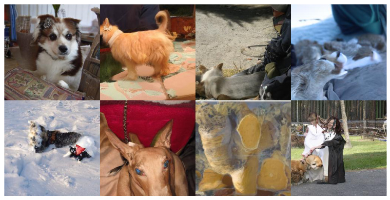
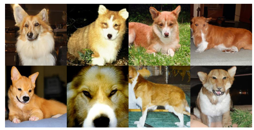
In early experiments with unconditional ImageNet models, a scale of exactly 1 was not enough. The classifier assigned reasonable probabilities — around 50% — to the desired class for the final samples, yet those samples did not match the intended class on visual inspection. Scaling the gradients up fixed it, and the class probabilities rose to nearly 100%.
What the scale means
The interpretation is exact, not a heuristic. Observe that
\[s\cdot\nabla_x\log p(y|x) = \nabla_x \log \tfrac{1}{Z}\,p(y|x)^s\]
for an arbitrary constant \(Z\). Scaling the gradient is therefore still theoretically grounded: it conditions on a re-normalised classifier distribution proportional to \(p(y|x)^s\). When \(s>1\) this distribution is sharper than \(p(y|x)\), since larger values are amplified by the exponent. A larger scale focuses on the modes of the classifier, which is desirable for higher fidelity and undesirable for diversity.
What the scale does
Figure 4 sweeps the scale for a class-conditional ImageNet \(128\times128\) model.
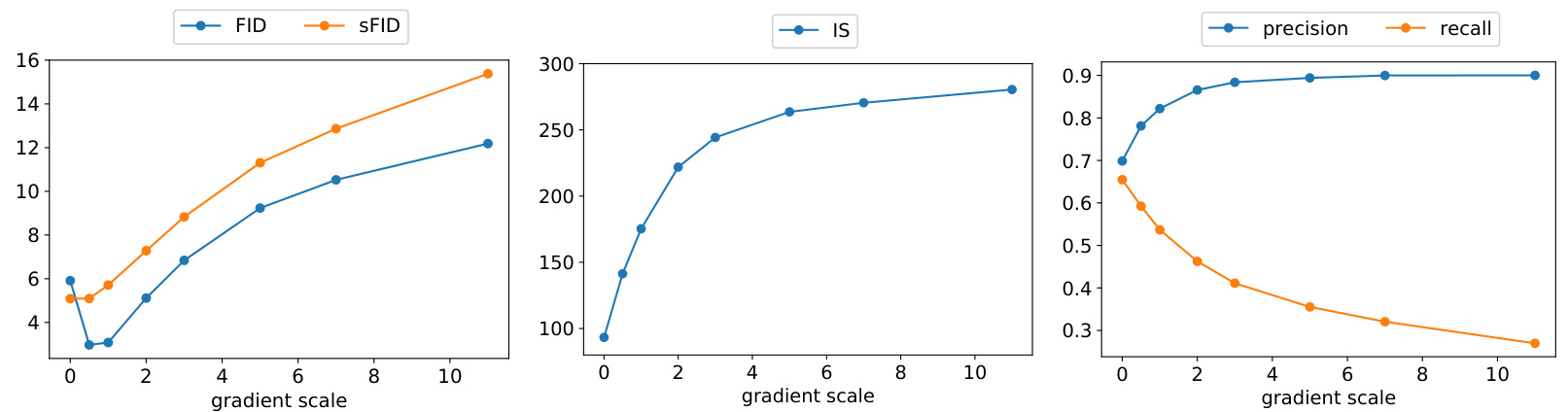
- Precision and IS rise monotonically with the scale; Recall falls monotonically.
- FID and sFID depend on both, so their best values sit at an intermediate point — near \(s = 0.5\) to \(1\) in this sweep, not at either extreme.
The paper’s Table 4, on ImageNet \(256\times256\), shows the same trade in numbers. An unconditional model has FID 26.21 and Recall 0.63; guided at scale 10.0 it reaches FID 12.00, IS 95.41, Precision 0.76 and Recall 0.44. A conditional model unguided has FID 10.94; guided at scale 1.0 it reaches 4.59. Two lessons follow.
- Guidance works on unconditional models too. A guided unconditional model gets close to an unguided conditional one, though training directly with labels still helps, and guiding a conditional model helps further.
- A result without its scale is not a result. The best \(s\) differs per metric and per resolution, so quoting a number requires quoting the scale that produced it.
The truncation analogy
This is the diffusion counterpart of BigGAN’s truncation trick, in which the latent is drawn from a truncated normal so that increased truncation lowers diversity and raises fidelity. Figure 5 puts the two side by side on ImageNet \(128\times128\).
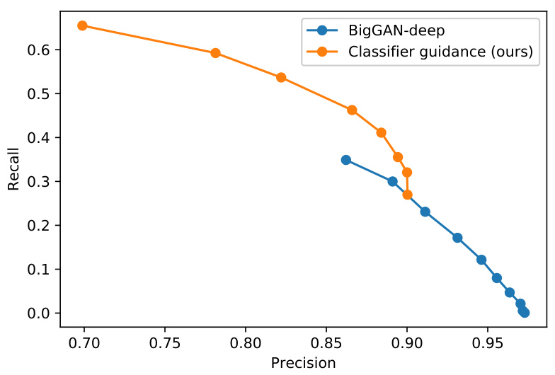
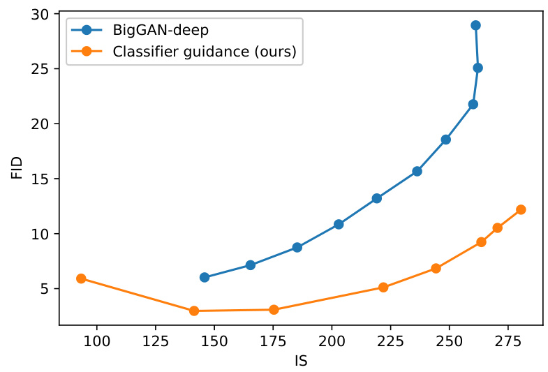
Classifier guidance is strictly better than BigGAN-deep when trading FID for Inception Score. The precision/recall picture is less clear cut: guidance is the better choice only up to a certain precision threshold, beyond which it cannot reach higher precision at all.
Learning outcomes
- gradient-scale-tradeoff Use the gradient scale to trade sample diversity for fidelity.
Concepts
- classifier-guidance explores practical classifier training and implementation details for guidance
- classifier-gradient-scale analyses the theoretical and empirical diversity/fidelity trade-off when tuning gradient scale \(s\)
What classifier guidance achieved
The architecture was evaluated on unconditional generation with three LSUN classes — bedroom, horse and cat — and guidance on class-conditional ImageNet at \(128\times128\), \(256\times256\) and \(512\times512\).
The headline
With the improved architecture alone, ADM already takes state of the art on LSUN and on ImageNet \(64\times64\). At higher ImageNet resolutions, classifier guidance carries it past the best GANs.
| Resolution | BigGAN-deep FID | ADM-G FID | BigGAN-deep Recall | ADM-G Recall |
|---|---|---|---|---|
| \(128\times128\) | 6.02 | 2.97 | 0.35 | 0.59 |
| \(256\times256\) | 6.95 | 4.59 | 0.28 | 0.52 |
| \(512\times512\) | 8.43 | 7.72 | 0.29 | 0.42 |
The second half of the table is the part that the truncation trick could not deliver. The guided models obtain perceptual quality similar to GANs while maintaining higher coverage of the distribution as measured by recall. Precision is a closer contest: at \(512\times512\) ADM-G reaches 0.87 against BigGAN-deep’s 0.88.
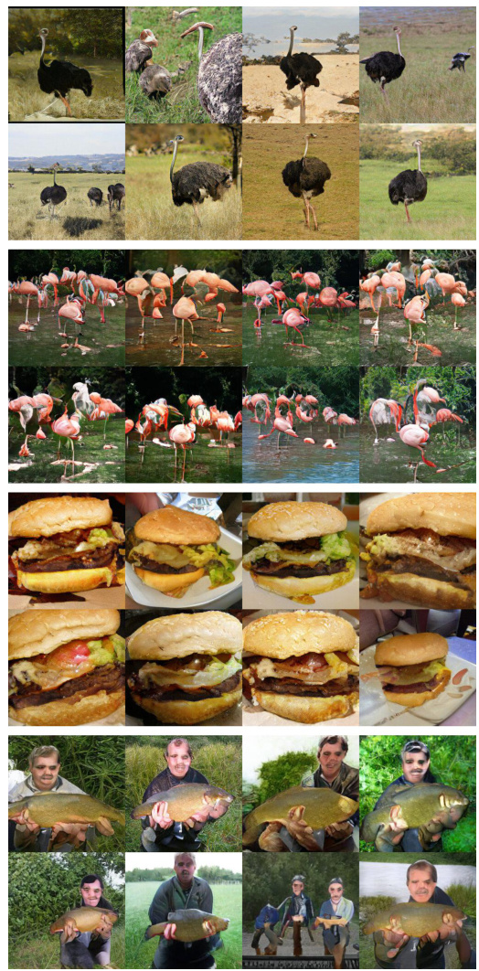
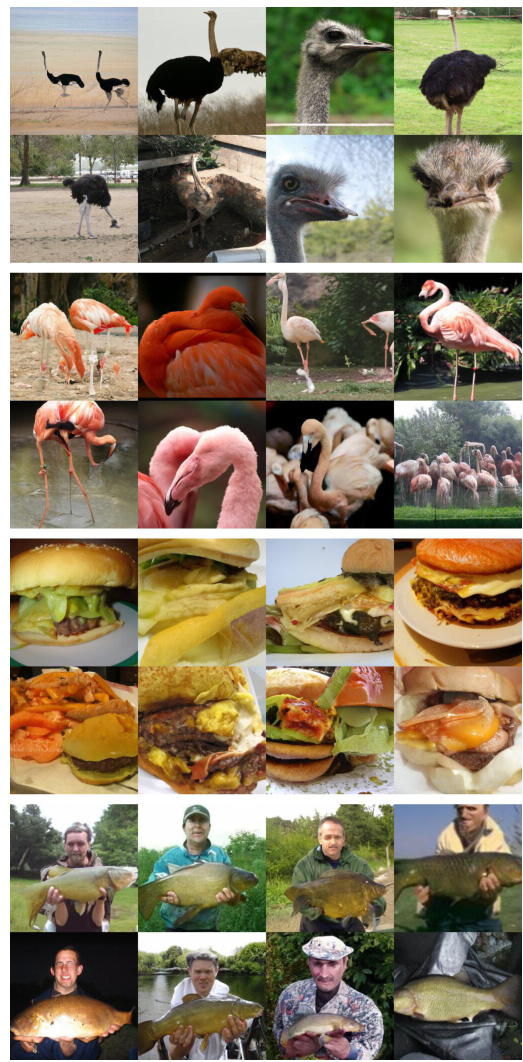
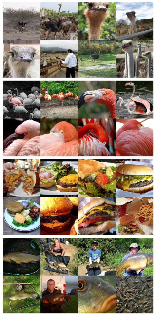
The samples are of similar perceptual quality, but the diffusion model contains more modes than the GAN — zoomed ostrich heads, single flamingos, different orientations of cheeseburgers, and a tinca fish with no human holding it.
Speed
Diffusion sampling is criticised for needing hundreds of sequential passes. Combined with DDIM at 25 steps, guidance still reaches ADM-G FID 5.98 at \(128\times128\) and 5.44 at \(256\times256\) — the latter beating BigGAN-deep’s 6.95 with Recall 0.49 against 0.28. That makes the comparison a fair one on compute, not only on quality.
Upsampling versus guidance
A two-stage upsampling stack (ADM-U) trains a separate diffusion model to super-resolve images, conditioning on the low-resolution image concatenated channel-wise after simple interpolation. The paper’s Table 6 shows the two techniques improve different things.
- Upsampling raises precision while keeping recall high.
- Guidance trades recall for much higher precision.
- Guiding the base model and then upsampling gives the best numbers of all: FID 3.94 at \(256\times256\) and 3.85 at \(512\times512\).
Three limitations are stated in the paper. Sampling remains slower than a GAN’s single forward pass, because of the multiple denoising steps. Classifier guidance is limited to labelled datasets, with no effective strategy offered for unlabelled ones. And the classifier must be trained specifically on noised inputs for this purpose.
That last pair of limitations is the opening for what follows. The paper itself names the way out: condition an image generator with a text caption using a noisy version of CLIP.
Learning outcomes
- classifier-guided-results Report what classifier-guided diffusion achieved against GANs, and at what cost.
Concepts
- ablated-diffusion-model reports benchmark results showing ADM beats previous models on unconditional LSUN and ImageNet \(64\times64\)
- classifier-guidance shows ADM with classifier guidance establishes state-of-the-art FID across ImageNet resolutions, and complements super-resolution upsamplers
- classifier-gradient-scale demonstrates that guided sampling achieves high visual quality with as few as 25 DDIM steps
- two-stage-upsampling-diffusion evaluates ADM-U and demonstrates record FIDs when combined with guidance
Text-conditional diffusion: GLIDE
GLIDE adopts the ADM architecture unchanged and augments it with text conditioning. For each noised image \(x_t\) and caption \(c\), the model predicts \(p(x_{t-1}|x_t, c)\). The change is small; the consequences are not.
How a caption enters the network
The caption is encoded into a sequence of \(K\) tokens, which are fed to a Transformer. The output is used in two ways.
The final token embedding is used in place of the class embedding in the ADM model.
That is the AdaGN path from the previous section. A single vector conditions every residual block globally, through the scale and shift.
The last layer of token embeddings — a sequence of \(K\) feature vectors — is separately projected to the dimensionality of each attention layer throughout the model, and concatenated to the attention context at that layer.
That is what lets individual spatial positions attend to individual words, so phrases rather than topics become controllable.
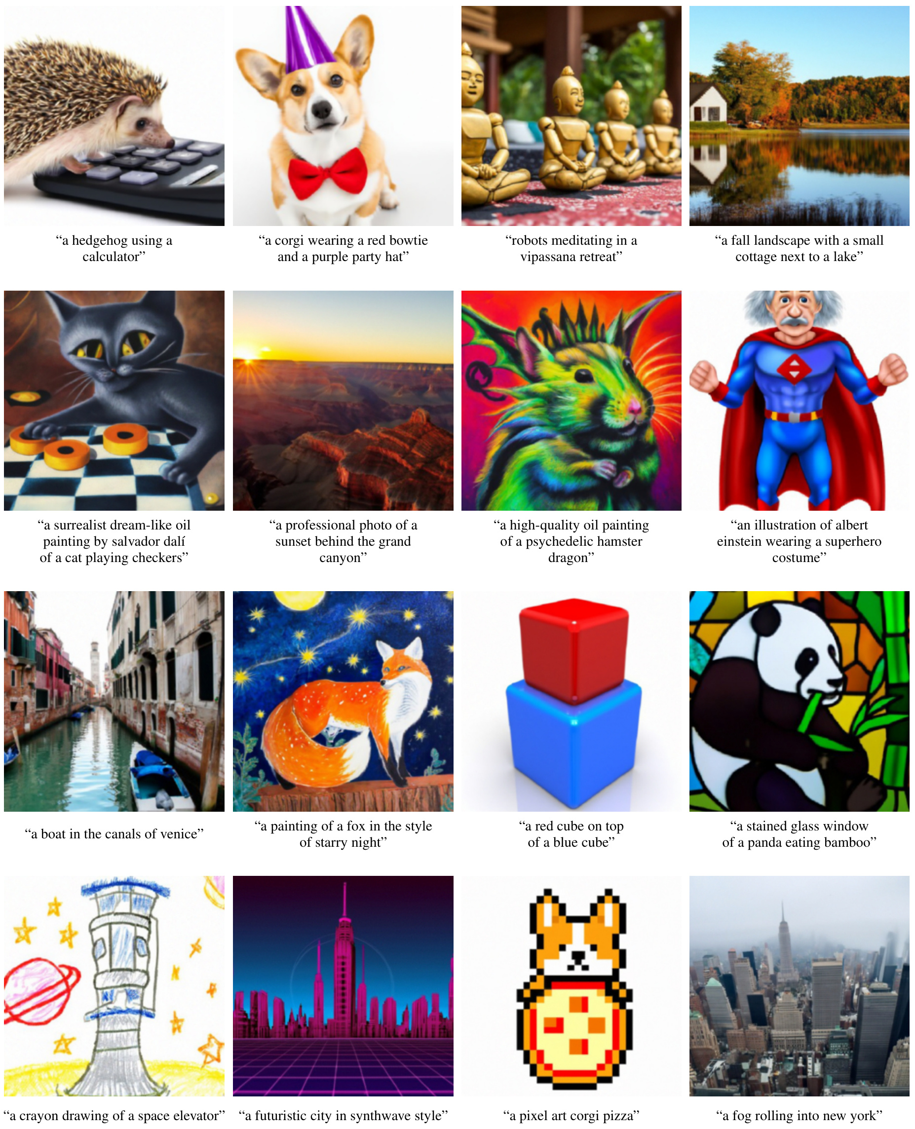
The paper observes in this figure that the model produces realistic shadows and reflections, composes multiple concepts in the correct way — a corgi, a bowtie and a birthday hat — while binding attributes such as colour to the right objects, and renders artistic styles from Salvador Dalí to pixel art.
Scale
- The base model runs at \(64\times64\) with roughly 3.5 billion parameters. The visual part is ADM with width scaled to 512 channels, about 2.3 billion parameters. The text encoder is a Transformer of 24 residual blocks at width 2048, about 1.2 billion.
- A separate 1.5 billion parameter upsampling model goes from \(64\times64\) to \(256\times256\). It is conditioned on text in the same way but with a smaller text encoder of width 1024, and otherwise matches the ImageNet upsampler of Dhariwal and Nichol with base channels increased to 384.
- Training used the same dataset as DALL-E. The base model was trained for 2.5M iterations at batch size 2048; the upsampler for 1.6M iterations at batch size 512. Both trained stably in 16-bit precision with traditional loss scaling. The total training compute is roughly equal to that used to train DALL-E.
Sampling uses 150 diffusion steps for the base model, 100 for inpainting, and 250 for FID evaluation. The upsampler uses a strided schedule of only 27 steps, split across five segments taking 10, 10, 3, 2 and 2 evenly-spaced steps — ten of them in the range \((0, 200]\) and only two in \((800, 1000]\).
This is the point at which the method becomes an engineering problem. Nothing in the recipe above is conceptually new; all of it is a matter of iterations, batch size and precision.
Learning outcomes
- text-conditional-diffusion Describe how GLIDE conditions a diffusion U-Net on free-form text.
Concepts
- glide details the core model architecture and training of GLIDE’s base and upsampler models
- glide-filtered lists the pre-training and fine-tuning iterations for the released filtered model
- noised-clip-guidance specifies the batch size, patch size and iterations for training the noised CLIP models
CLIP guidance with a noised CLIP
CLIP consists of an image encoder \(f(x)\) and a caption encoder \(g(c)\), trained on batches of \((x, c)\) pairs with a contrastive cross-entropy loss that encourages a high dot product \(f(x)\cdot g(c)\) when image and caption are paired, and a low one when they are not.
That dot product is a score of how close an image is to a caption. Classifier guidance needs nothing more than such a score, differentiable in \(x\). So replace the classifier with CLIP and perturb the reverse-process mean by the gradient of the dot product with respect to the image:
\[\hat\mu_\theta(x_t|c) = \mu_\theta(x_t|c) + s\cdot\Sigma_\theta(x_t|c)\,\nabla_{x_t}\big(f(x_t)\cdot g(c)\big)\]
Set beside the classifier form from the previous section,
\[\hat\mu_\theta(x_t|y) = \mu_\theta(x_t|y) + s\cdot\Sigma_\theta(x_t|y)\,\nabla_{x_t}\log p_\phi(y|x_t)\]
the substitution is exactly one term. What it buys is that \(c\) may be any caption, and no labelled dataset is required.
The catch, and the fix
A CLIP model trained on clean photographs is being asked to score \(x_t\), which during sampling is a heavily noised image. Those inputs are out of distribution for it, and the paper hypothesises that this is precisely why guiding with a public CLIP model adversely affects sample quality.
The fix is noised CLIP: train the image encoder as \(f(x_t, t)\), receiving noised images directly, otherwise with the same objective as the original CLIP model. GLIDE’s models are trained at \(64\times64\) resolution with the same noise schedule as the base diffusion model. The noised CLIP models process \(64\times64\) images with a ViT at patch size \(4\times4\), trained for 390K iterations at batch size 32K on a 50–50 mixture of the CLIP and DALL-E datasets; the final ViT-L used weight decay 0.0125 and was then fine-tuned for 30K iterations on a broader dataset of internet images.
Does the noise-awareness matter?
Appendix D answers this directly. A popular public CLIP-guided diffusion program requires a set of engineered augmentations and auxiliary perceptual losses to get recognisable samples at all. The paper’s comparison uses a noised ViT-B CLIP to guide the ImageNet \(64\times64\) model of Dhariwal and Nichol at a fixed gradient scale of 15.0, selecting a different random class label at each timestep since that model is class-conditional, then upsamples to \(256\times256\).
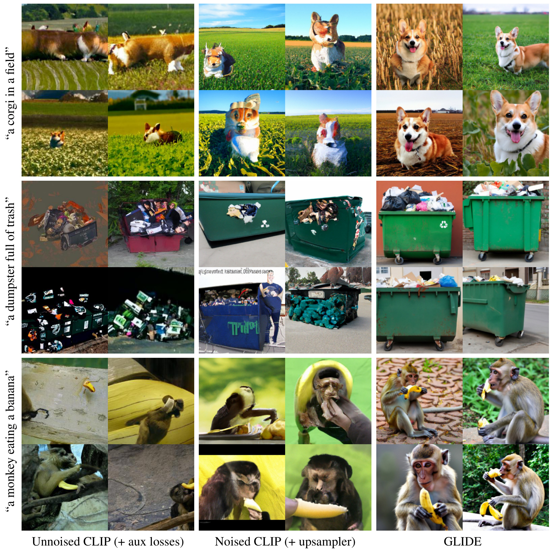
The noise-aware approach produces images of equal or higher quality despite being much simpler, which the paper reads as evidence that making CLIP noise-aware is indeed helpful.
A second large model, with a backward pass at every sampling step, plus its own training run of 390K iterations at batch size 32K. The labelled dataset is gone; the second network is not.
Learning outcomes
- clip-guidance Guide a diffusion model with a CLIP score, using a noise-aware CLIP.
Concepts
- noised-clip-guidance formulates CLIP guidance using gradients from a CLIP model trained on noised images, and specifies its training setup
Comparing guidance strategies
We now have two ways to steer a text-conditional diffusion model, and a clean question: which is better? The answer depends on who is asked, and that dependence is the lesson.
The competitor
Classifier-free guidance requires no separate model. During training the label is replaced with a null label \(\emptyset\) with fixed probability; GLIDE fine-tunes its base model after pre-training with 20% of text token sequences replaced by the empty sequence, so the model retains conditional generation while also generating unconditionally. At sampling time the prediction is extrapolated away from the unconditional one:
\[\hat\epsilon_\theta(x_t|c) = \epsilon_\theta(x_t|\emptyset) + s\cdot\big(\epsilon_\theta(x_t|c) - \epsilon_\theta(x_t|\emptyset)\big)\]
with \(s \ge 1\) the guidance scale. Two properties make it appealing: a single model leverages its own knowledge rather than that of a separate and sometimes smaller classifier, and it simplifies guidance when the conditioning information is hard to predict with a classifier — text being exactly such a case. We use it operationally here; the derivation belongs to the next unit.
The automated verdict
Both approaches were swept on zero-shot MS-COCO generation at \(64\times64\).
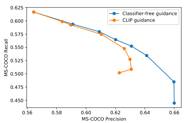
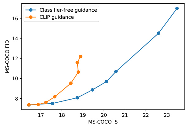
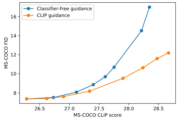
Classifier-free guidance is nearly Pareto optimal on FID against IS and on Precision against Recall. On CLIP score against FID the trend reverses exactly: CLIP guidance boosts CLIP score far more than classifier-free guidance does.
The human verdict
Human evaluators were shown two \(256\times256\) images and asked which better matches the caption, or which looks more photorealistic, with the option to say neither is significantly better — a tie counting as half a win for each model. One thousand pairwise comparisons were collected per setting for photorealism, and one thousand for caption similarity, except in guidance-scale sweeps where five hundred sufficed. Elo scores \(\sigma_i\) were fitted by minimising
\[\mathcal{L}_{\mathrm{elo}} := -\sum_{i,j} A_{ij}\cdot\log\left(\frac{1}{1 + 10^{(\sigma_i-\sigma_j)/400}}\right)\]
where \(A_{ij}\) counts the times model \(i\) beat model \(j\). Guidance scales were swept separately for each method first, then the best of each compared.
| Guidance | Photorealism | Caption |
|---|---|---|
| Unguided | -88.6 | -106.2 |
| CLIP guidance (scale 2.0) | -73.2 | 29.3 |
| Classifier-free guidance (scale 3.0) | 82.7 | 110.9 |
Humans disagree with the CLIP score. The method that wins on CLIP score loses decisively on both human axes, including on caption similarity — the very thing the CLIP score purports to measure. The paper’s hypothesis is that CLIP guidance is finding adversarial examples for the evaluation CLIP model, rather than actually matching the prompt better.
Do not evaluate a method with the same objective it optimises. CLIP guidance ascends the CLIP score by construction; that a CLIP score results is not evidence of anything.
Against DALL-E
Automated evaluation used 30,000 samples from MS-COCO validation prompts with the entire validation set as reference, and center-cropped validation images rather than the squeezing common in text-conditional work. CLIP score used the public CLIP ViT-B/16 scaled by the CLIP logit scale of 100.
GLIDE obtains a zero-shot FID of 12.24 on MS-COCO \(256\times256\) at classifier-free guidance scale 1.5, rising slightly to 12.89 against a validation subset purged of images similar to the training set — a change the paper attributes largely to FID bias from the smaller reference batch. Against DALL-E, at 3.5 billion parameters versus 12 billion and roughly the same training compute, GLIDE is preferred by human evaluators in every setting: 87% on photorealism and 69% on caption similarity against DALL-E reranked at temperature 0.85, and still 66% and 61% when GLIDE’s own samples are deliberately blurred through DALL-E’s discrete VAE.
Learning outcomes
- comparing-guidance-strategies Compare CLIP guidance against classifier-free guidance and explain why the CLIP score misleads.
Concepts
- classifier-free-guidance defines the formulation, the fine-tuning that enables it, and its Pareto optimality and human-evaluation dominance
- noised-clip-guidance evaluates CLIP guidance performance and explains its inflated CLIP scores
- glide reports benchmark FIDs and direct human win rates of GLIDE against DALL-E
Inpainting and editing
A model that renders a prompt zero-shot can still fail on a complex one. Editing is the remedy: let the user refine a sample until it matches. The mechanism is simpler than the capability suggests.
The naive approach, and why it falls short
Most previous work did not train diffusion models for inpainting at all. Instead, inpainting is performed by sampling from the model as usual, but replacing the known region of the image with a sample from \(q(x_t|x_0)\) after each sampling step.
The disadvantage is structural: the model never sees the entire context during sampling, only a noised version of it. In the authors’ early experiments this occasionally produced undesired edge artifacts.
Explicit fine-tuning
The fix is to fine-tune for the task. During fine-tuning, random regions of training examples are erased, and the remaining portions are fed to the model along with a mask channel as additional conditioning information. The architecture gains four additional input channels:
- a second set of RGB channels, carrying the unmasked context;
- one mask channel.
The corresponding input weights for these new channels are initialised to zero before fine-tuning, so the fine-tune begins from exactly the pre-trained model’s behaviour. For the upsampling model, the full low-resolution image is always provided, but only the unmasked region of the high-resolution image.
What it enables
- Realistic insertions. The model inserts new objects, shadows and reflections where needed, matching the style and lighting of the surrounding context, and can match styles when editing objects into paintings.
- Iterative scene construction. A zero-shot generation followed by a series of masked prompts — a painting on the wall, a coffee table, a vase of flowers on the table, then the wall moved up to the couch — builds a complex scene one edit at a time.
- Sketch to image. With SDEdit, the user combines a rough sketch with a caption to make controlled modifications, such as adding a bow tie and birthday hat to a corgi.
Fine-tuning versus implicit conditioning
Appendix E evaluates GLIDE against Blended Diffusion, which uses CLIP-guided editing without task-specific fine-tuning.
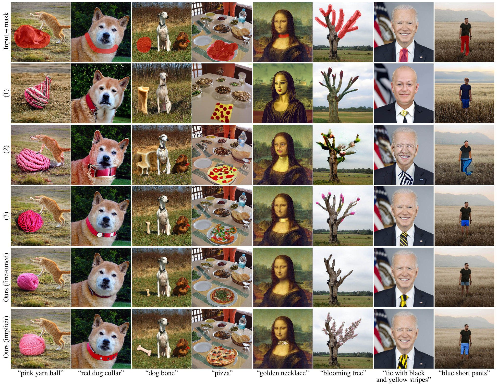
The comparison is not one-sided, and this is worth noticing. The fine-tuned model has more realistic lighting, shadows and textures, but sometimes chooses to ignore the given text prompt and produces an image influenced only by the surrounding context — the “golden necklace” column is the example the paper points to. Running the same model with the context fully masked out, so that it receives context only through the noised masked \(x_t\), makes it follow the caption more consistently, at the cost of producing objects that fit less smoothly into the scene.
Key ideas
- Inpainting needs no new architecture, only four input channels and a fine-tuning run.
- Zero-initialised weights on the new channels mean fine-tuning starts from the pre-trained behaviour.
- Explicit fine-tuning buys blending; implicit conditioning buys prompt adherence.
Learning outcomes
- inpainting-and-editing Fine-tune a text-conditional diffusion model for text-guided inpainting and editing.
Concepts
- text-conditional-inpainting details the addition of mask and context RGB channels to enable high-quality text-driven image editing
- glide documents the fine-tuning of GLIDE’s base and upsampler diffusion models on inpainting tasks
Safety, filtering and limitations
The deployment reasoning here is part of the method, not an appendix to it. The paper states the risk plainly: the model produces fake but realistic images and enables unskilled users to make convincing edits to existing images, so releasing it without safeguards would significantly reduce the skills required to create convincing disinformation or deepfakes. Its samples also reflect biases, including those of the dataset.
Filtering the data
Several hundred million images were gathered from the internet, largely disjoint from the datasets used to train CLIP and DALL-E, and then filtered.
People. Several thousand boolean labels were collected on random training samples. Each image was resized so the smaller side is 224 pixels, three crops taken along the longer side, all three fed through a pre-trained CLIP ViT-B/16, and the feature vectors mean-pooled. An SVM with an RBF kernel was fitted, with the bias tuned for under a 1% false negative rate. On a separate batch of 1024 samples it produced no false negatives.
An earlier attempt using ViT-B/32 missed people in low-light or obstructed conditions. The higher hidden-state resolution of ViT-B/16 remedied every observed failure case.
Violent objects. CLIP was used to search for words like “weapon” and “violence”, then an SVM trained, then samples near its decision boundary labelled and the process iterated — active learning — before tuning the bias to the same 1% target.
Hate symbols. The keyword search surfaced very few relevant images, suggesting the data sources had already filtered such content. Images of the swastika and the Confederate flag were collected by search engine and an SVM trained on them.
A 300 million parameter model, GLIDE (filtered), was trained on the filtered data — 1.1M pre-training iterations plus 500K of fine-tuning for classifier-free guidance and inpainting. Red-teaming with adversarial prompts found no instance where it generated a recognisable image of a human.
Filtering does not remove bias
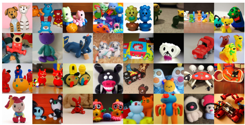
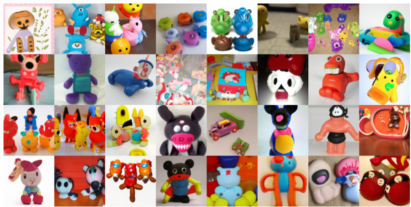
The filtered model retains, and may amplify, biases in the dataset. Asked for “toys for girls” it produces more pink toys and stuffed animals than for “toys for boys”. Asked for “a religious place” it gravitates toward church-like buildings, and this bias is amplified by classifier-free guidance. The hate-symbol filter is acknowledged to carry a strong American and Western bias, having been trained on two symbols only.
Filtering also costs capability in unexpected places: GLIDE (filtered) renders “orange triangle” and “recycling symbol” less faithfully than the unfiltered GLIDE (small), although neither symbol was filtered — likely a consequence of the smaller dataset.
No model lives in a vacuum
Swapping GLIDE (filtered) into a publicly available CLIP-guided diffusion program gave the pair some ability to generate face-like objects, and some hateful imagery. The mitigating observation is that the same public CLIP model produced roughly the same quality of images when paired with a publicly available ImageNet diffusion model. The point stands as a limitation of the filtering approach: capabilities compose across models even when they were removed from one.
What remains hard
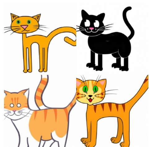
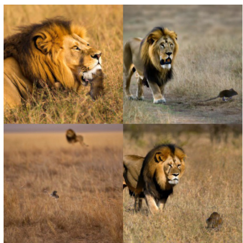
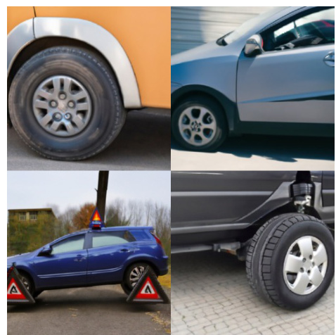
- Unusual compositions fail. The model composes disparate concepts well, but sometimes fails on prompts describing highly unusual objects or scenarios.
- Sampling is slow. The unoptimised model takes 15 seconds to sample one image on a single A100 GPU, much slower than GAN methods that produce an image in a single forward pass, and therefore less favourable for real-time applications.
Learning outcomes
- safety-and-limitations Assess the safety case for releasing a text-to-image model, and what these models still cannot do.
Concepts
- glide-filtered describes the dataset filtering pipeline and audits the societal biases and external-CLIP vulnerabilities that survive it
- classifier-free-guidance shows that increasing the guidance scale exacerbates cultural and religious biases
- noised-clip-guidance examines the effect of guiding the filtered model with external CLIP models
Towards classifier-free guidance
Two papers, one recipe. Dhariwal and Nichol conclude that diffusion models — likelihood- based models with a stationary training objective — can obtain better sample quality than state-of-the-art GANs; that improved architecture alone suffices for unconditional generation; that classifier guidance supplies the conditional case with a scale that trades diversity for fidelity; and that guidance combined with upsampling improves high-resolution synthesis further. GLIDE’s abstract carries the sequel: applied to text-conditional synthesis, classifier-free guidance is preferred by human evaluators over CLIP guidance on both photorealism and caption similarity, a 3.5 billion parameter model beats DALL-E even when the latter uses expensive CLIP reranking, and the same model fine-tunes into a text-driven image editor.
What to carry away
Conditioning the reverse step on \(c\) shifts the Gaussian mean by \(\Sigma\nabla_{x_t}\log p_\phi(c|x_t)\) and leaves the covariance alone.
That is why guidance costs one backward pass per step and nothing else.
Scaling that gradient by \(s\) samples from a renormalised \(p(y|x)^s\).
A single exact identity turns a hyperparameter into a fidelity-versus-diversity knob with a known meaning.
The classifier — or CLIP — must be trained on noised images.
It is evaluated on \(x_t\), so anything trained only on clean images is being asked for gradients where it has never looked.
Much of the gain came from the backbone, not the guidance.
Measure the ablation before crediting the method.
CLIP guidance wins on CLIP score and loses to humans on both photorealism and caption similarity.
Optimising a metric hard enough finds adversarial examples for it. The warning raised in 2021 Clip is here demonstrated concretely.
Filtering removes capabilities, not biases.
It can amplify the biases that remain, and capabilities recompose when the filtered model is paired with an unfiltered one.
Both methods in this unit need a second network — a noised classifier, or a noised CLIP — and each brings extra training, extra memory, and a backward pass per sampling step. The next unit, 2022 Classifier Free Diffusion Guidance, shows this is unnecessary. Drop the conditioning signal for a small fraction of training and one model supplies both the conditional and the unconditional score; extrapolating between them at a strength \(w\) reproduces the whole trade-off curve. We have used that method operationally here, taking its formula on trust; next we derive it and study the \(w\) sweep properly.
Learning outcomes
- metrics-and-architecture Evaluate diffusion samples with the standard metrics and describe the U-Net changes that improved them.
- classifier-guidance-derivation Derive the classifier-guided reverse step and its DDIM counterpart.
- gradient-scale-tradeoff Use the gradient scale to trade sample diversity for fidelity.
- classifier-guided-results Report what classifier-guided diffusion achieved against GANs, and at what cost.
- text-conditional-diffusion Describe how GLIDE conditions a diffusion U-Net on free-form text.
- clip-guidance Guide a diffusion model with a CLIP score, using a noise-aware CLIP.
- comparing-guidance-strategies Compare CLIP guidance against classifier-free guidance and explain why the CLIP score misleads.
- inpainting-and-editing Fine-tune a text-conditional diffusion model for text-guided inpainting and editing.
- safety-and-limitations Assess the safety case for releasing a text-to-image model, and what these models still cannot do.
References
Dhariwal, P., & Nichol, A. (2021). Diffusion models beat gans on image synthesis. Advances in neural information processing systems, 34, 8780-8794.
Nichol, Alex, et al. “Glide: Towards photorealistic image generation and editing with text-guided diffusion models.” arXiv preprint arXiv:2112.10741 (2021).