Lecture notes — 2 Working with text data
ver. 1.2.0, 2_working_with_text_data
ver. 1.2.0 · 2026-09-02 16:28:17
Where this fits
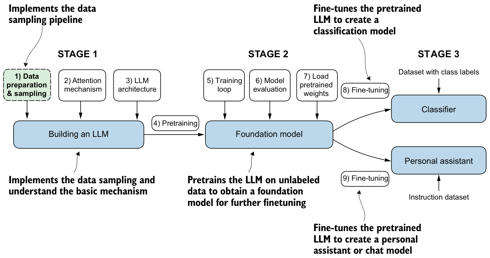
The previous unit, 1 Understanding large language models, established that a GPT-style model is a decoder-only transformer trained by next-word prediction, and laid out a three-stage roadmap: build the architecture, pretrain a foundation model, then fine-tune it. This unit is step 1 of stage 1.
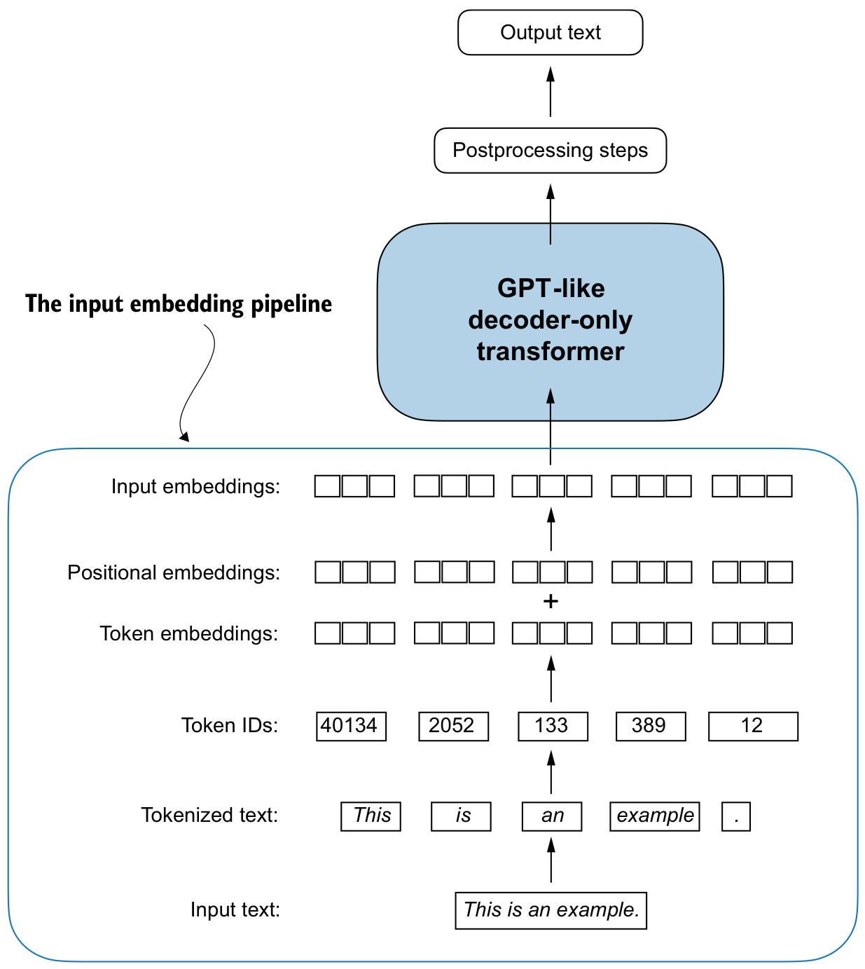
A transformer accepts a tensor of continuous-valued vectors. A corpus is a string. The distance between the two is four operations — split the text into tokens, map the tokens to integers, look up a vector for each integer, and add a vector that records position — and the unit closes with a PyTorch DataLoader that performs all four and yields the exact tensor the model of the next unit consumes.
Learning outcomes
explain-embeddings— Explain why text must become continuous vectors, and what an embedding is.tokenize-raw-text— Split raw text into tokens with a regular expression, and justify the choices that split makes.build-vocabulary-and-tokenizer— Build a vocabulary and a tokenizer class with matchingencodeanddecodemethods.handle-unknown-tokens— Extend a vocabulary with special context tokens to handle unseen words and document boundaries.apply-byte-pair-encoding— Use byte pair encoding to tokenize arbitrary text without an out-of-vocabulary failure.build-sliding-window-dataloader— Generate input–target pairs for next-token prediction with a sliding window, and load them in batches.create-token-embeddings— Turn token IDs into vectors with annn.Embeddinglayer, and explain what that layer really is.add-positional-embeddings— Add absolute positional embeddings to token embeddings to produce the model’s final input.
Concepts introduced
- Word embeddings — continuous-valued vector representations of discrete tokens, parameterized by a weight matrix and learned during training.
- Tokenization — the splitting of raw text into individual units: words, punctuation characters, or subwords.
- Vocabulary and token IDs — a bijection between the set of unique tokens and a set of integers, held as two dictionaries that invert one another.
- Special context tokens — entries added to a vocabulary that carry structural information rather than text:
<|unk|>,<|endoftext|>,[BOS],[EOS],[PAD]. - Byte pair encoding — a subword tokenization scheme whose vocabulary is built by iteratively merging frequent adjacent symbols, starting from single characters.
- Sliding window data sampling — the extraction of input and target sequences from a token stream, where the target is the input advanced by one position.
- Positional embeddings — vectors indexed by position in the sequence, added to token embeddings so that order is represented in the input.
Why text has to become vectors
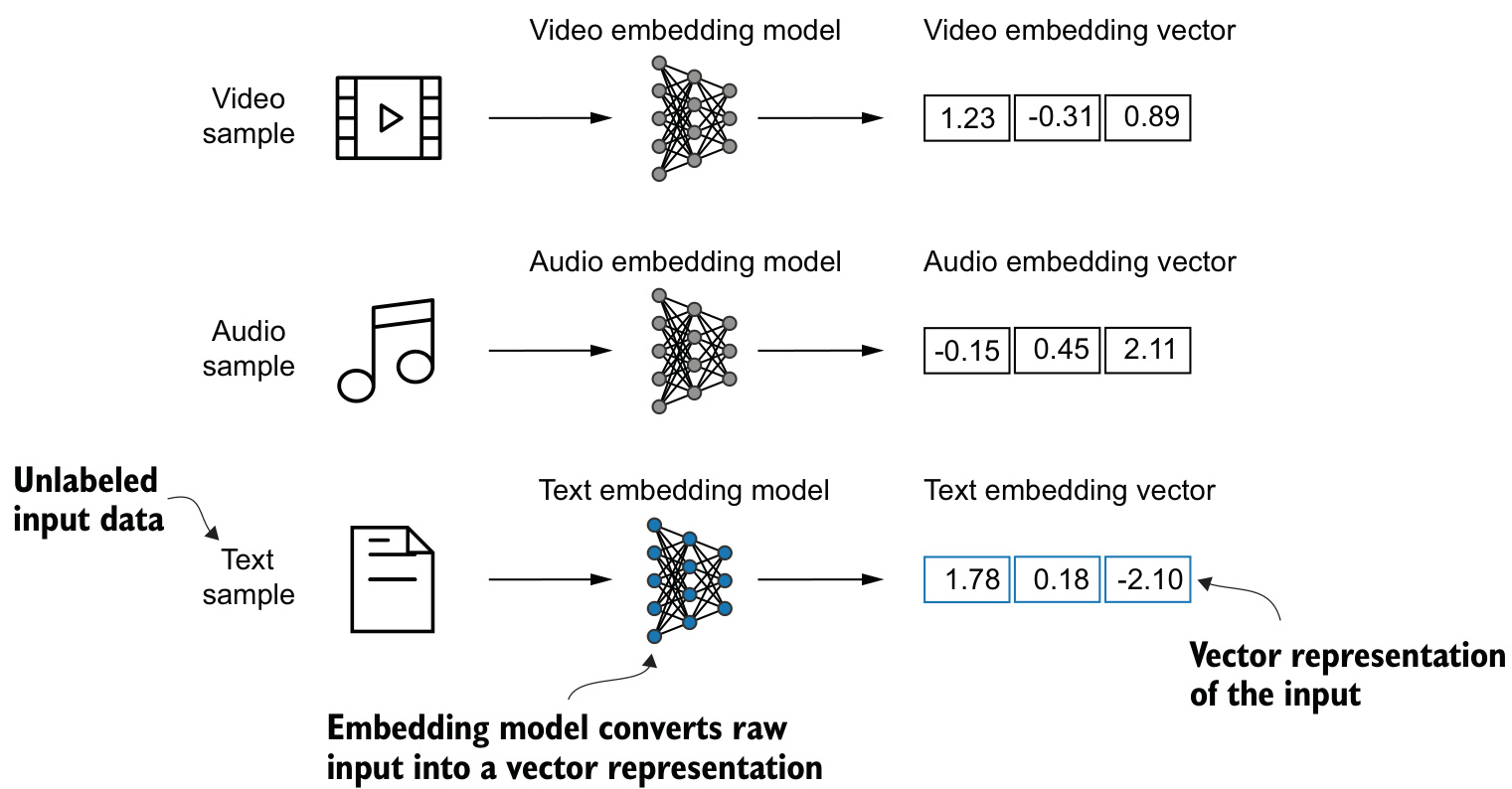
Deep neural network models, LLMs among them, cannot process raw text directly. Text is categorical, and categorical data is not compatible with the mathematical operations used to implement and train neural networks. Words must therefore be represented as continuous-valued vectors.
The conversion of data into a vector format is called embedding. At its core, an embedding is a mapping from discrete objects — words, images, or even entire documents — to points in a continuous vector space. Its primary purpose is to convert nonnumeric data into a format neural networks can process.
Different data formats require distinct embedding models. An embedding model designed for text is not suitable for embedding audio or video data, even though the output in each case is a vector of the same kind.
Word embeddings are the most common form of text embedding, but embeddings also exist for sentences, paragraphs and whole documents. Sentence and paragraph embeddings are popular choices for retrieval-augmented generation, which combines generation with retrieval from an external knowledge base. Since the goal here is a GPT-like model that generates one word at a time, the work is at the word level.
Standalone embeddings and in-model embeddings
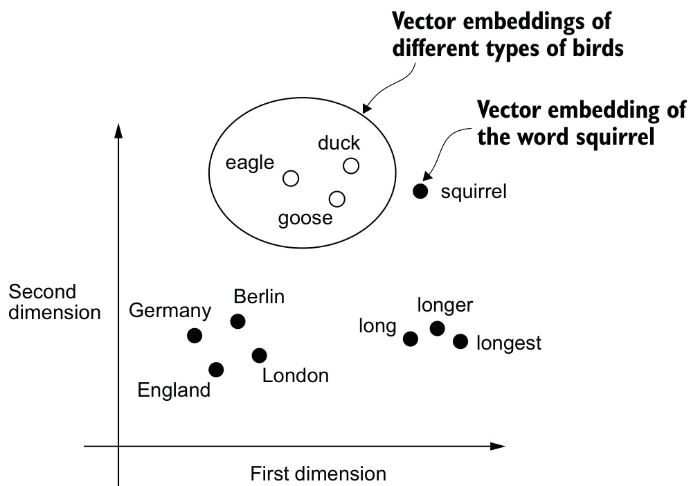
Several algorithms produce word embeddings on their own. Word2Vec trains a neural network architecture to generate word embeddings by predicting the context of a word given the word, or the word given its context. Its premise is that words appearing in similar contexts tend to have similar meanings; projected to two dimensions for visualization, similar terms cluster together.
LLMs do not use Word2Vec vectors. They produce their own embeddings, which are part of the input layer and are updated during training. The advantage is that the embeddings are optimized to the specific task and data at hand rather than to a separate proxy objective.
Dimensionality is a design choice, and a tradeoff between performance and efficiency:
The smallest GPT-2 models (117M and 125M parameters) use an embedding size of 768 dimensions.
A higher dimensionality might capture more nuanced relationships, at the cost of computational efficiency.
The largest GPT-3 model (175B parameters) uses an embedding size of 12,288 dimensions.
The embedding size is often referred to as the dimensionality of the model’s hidden states, and it varies with the model variant.
Embeddings can have anywhere from one to thousands of dimensions. Human sensory perception and common graphical representations are limited to three dimensions or fewer, which is why figure 2.3 shows a two-dimensional case.
Learning outcomes
- explain-embeddings Explain why text must become continuous vectors, and what an embedding is.
Concepts
- word-embeddings a discrete token is mapped to a dense vector in a continuous space, which is the only form of input a neural network can operate on
Tokenizing text
The text tokenized throughout the chapter is “The Verdict,” a short story by Edith Wharton that has been released into the public domain. Listing 2.1 reads it in:
with open("the-verdict.txt", "r", encoding="utf-8") as f:
    raw_text = f.read()
print("Total number of character:", len(raw_text))
print(raw_text[:99])
Total number of character: 20479
I HAD always thought Jack Gisburn rather a cheap genius--though a good fellow
enough--so it was noTokenization splits this 20,479-character string into individual words and special characters. The split is built up with Python’s re module, one decision at a time. Splitting on whitespace characters alone:
import re
text = "Hello, world. This, is a test."
result = re.split(r'(\s)', text)
print(result)
['Hello,', ' ', 'world.', ' ', 'This,', ' ', 'is', ' ', 'a', ' ', 'test.']Words are separated, but Hello, and world. are still joined to punctuation characters that should be separate entries. Adding commas and periods to the pattern separates them:
result = re.split(r'([,.]|\s)', text)
print(result)
['Hello', ',', '', ' ', 'world', '.', '', ' ', 'This', ',', '', ' ', 'is',
' ', 'a', ' ', 'test', '.', '']The split now emits empty strings and whitespace entries. Both are removed by a list comprehension that keeps only items with non-whitespace content:
result = [item for item in result if item.strip()]
print(result)
['Hello', ',', 'world', '.', 'This', ',', 'is', 'a', 'test', '.']Whether whitespace should be encoded as separate characters or removed depends on the application. Removing whitespace reduces the memory and computing requirements. Keeping it matters for models that are sensitive to the exact structure of the text — Python code, for instance, is sensitive to indentation and spacing. It is removed here for brevity; the tokenization scheme adopted later in the chapter includes whitespace.
Text is not lower-cased. Capitalization helps an LLM distinguish between proper nouns and common nouns, understand sentence structure, and learn to generate text with proper capitalization.
The final pattern adds question marks, quotation marks, the remaining punctuation and the double dash:
text = "Hello, world. Is this-- a test?"
result = re.split(r'([,.:;?_!"()\']|--|\s)', text)
result = [item.strip() for item in result if item.strip()]
print(result)
['Hello', ',', 'world', '.', 'Is', 'this', '--', 'a', 'test', '?']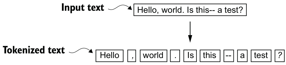
Applied to the whole short story, the same two lines produce a list of token strings:
preprocessed = re.split(r'([,.:;?_!"()\']|--|\s)', raw_text)
preprocessed = [item.strip() for item in preprocessed if item.strip()]
print(len(preprocessed))
The print statement outputs 4690, the number of tokens in the text without whitespaces. The first thirty confirm that words and special characters are neatly separated:
['I', 'HAD', 'always', 'thought', 'Jack', 'Gisburn', 'rather', 'a',
'cheap', 'genius', '--', 'though', 'a', 'good', 'fellow', 'enough',
'--', 'so', 'it', 'was', 'no', 'great', 'surprise', 'to', 'me', 'to',
'hear', 'that', ',', 'in']Learning outcomes
- tokenize-raw-text Split raw text into tokens with a regular expression, and justify the choices that split makes.
Concepts
- tokenization raw text is broken into words and punctuation characters by an explicit regular expression, and every character class in that expression is a decision about what counts as a unit
From tokens to token IDs
The tokens are still Python strings. Converting them to an integer representation produces the token IDs, an intermediate step before the embedding vectors. The mapping is defined by a vocabulary: every unique word and special character is assigned a unique integer.
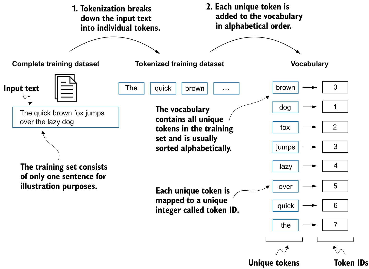
all_words = sorted(set(preprocessed))
vocab_size = len(all_words)
print(vocab_size)
The vocabulary size is 1,130 — fewer than the 4,690 tokens, because duplicates are removed. Listing 2.2 builds the dictionary:
vocab = {token:integer for integer,token in enumerate(all_words)}
for i, item in enumerate(vocab.items()):
    print(item)
    if i >= 50:
        break
('!', 0)
('"', 1)
("'", 2)
...
('Her', 49)
('Hermia', 50)Reading the model’s numerical output back as text requires the inverse dictionary, mapping token IDs to their token strings. Listing 2.3 packages both directions in one class:
class SimpleTokenizerV1:
    def __init__(self, vocab):
        self.str_to_int = vocab
        self.int_to_str = {i:s for s,i in vocab.items()}

    def encode(self, text):
        preprocessed = re.split(r'([,.?_!"()\']|--|\s)', text)
        preprocessed = [
            item.strip() for item in preprocessed if item.strip()
        ]
        ids = [self.str_to_int[s] for s in preprocessed]
        return ids

    def decode(self, ids):
        text = " ".join([self.int_to_str[i] for i in ids])

        text = re.sub(r'\s+([,.?!"()\'])', r'\1', text)
        return text
The re.sub call in decode is the step that is easiest to get wrong. Joining tokens with " ".join inserts a space before every token, including punctuation, which yields pride . instead of pride.. The substitution removes whitespace that directly precedes one of the listed punctuation characters, and nowhere else.
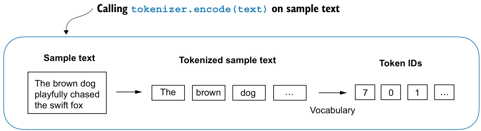
encode takes sample text, splits it into tokens, and converts the tokens into token IDs via the vocabulary.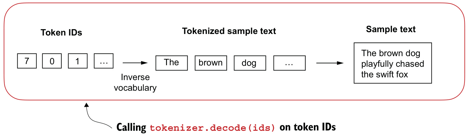
decode takes token IDs, converts them back into text tokens through the inverse vocabulary, and concatenates them into natural text.Applied to a passage from the story:
tokenizer = SimpleTokenizerV1(vocab)
text = """"It's the last he painted, you know,"
       Mrs. Gisburn said with pardonable pride."""
ids = tokenizer.encode(text)
print(ids)
[1, 56, 2, 850, 988, 602, 533, 746, 5, 1126, 596, 5, 1, 67, 7, 38, 851, 1108,
754, 793, 7]print(tokenizer.decode(ids))'" It\' s the last he painted, you know," Mrs. Gisburn said with
pardonable pride.'The round trip returns the original text, which is the check that catches a mismatch between encode and decode. Applied to text from outside the training set, however, encode fails:
text = "Hello, do you like tea?"
print(tokenizer.encode(text))
KeyError: 'Hello'The word “Hello” was not used in “The Verdict,” so it is not in the vocabulary, and the dictionary lookup in encode raises. A closed vocabulary built from one text cannot encode arbitrary text.
Learning outcomes
- build-vocabulary-and-tokenizer Build a vocabulary and a tokenizer class with matching
encodeanddecodemethods.
Concepts
- vocabulary-and-token-ids the unique tokens sorted alphabetically and numbered from zero give
str_to_int, and inverting that dictionary givesint_to_str - tokenization the same regular-expression split that produced the token list is what
encodeapplies to new text before the integer lookup
Special context tokens
Two additions to the vocabulary fix two distinct failures. SimpleTokenizerV2 supports both.
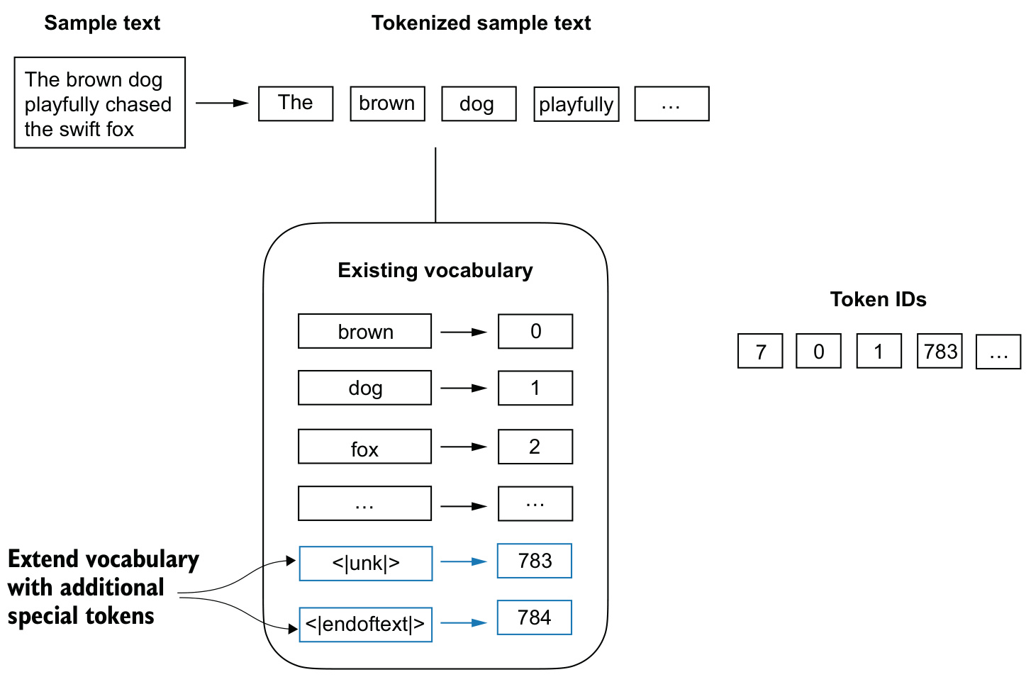
<|unk|> represents words that were not part of the training data, and <|endoftext|> separates two unrelated text sources.<|unk|>is substituted for any token that is not in the vocabulary, soencodereturns an ID rather than raising aKeyError.The word itself is lost. What survives is the position and the fact that a token stood there.
<|endoftext|>is inserted between independent documents when a corpus is concatenated.When training on multiple independent documents or books, it is common to insert this token before each document that follows a previous text source. This helps the model understand that although the sources are concatenated for training, they are in fact unrelated.
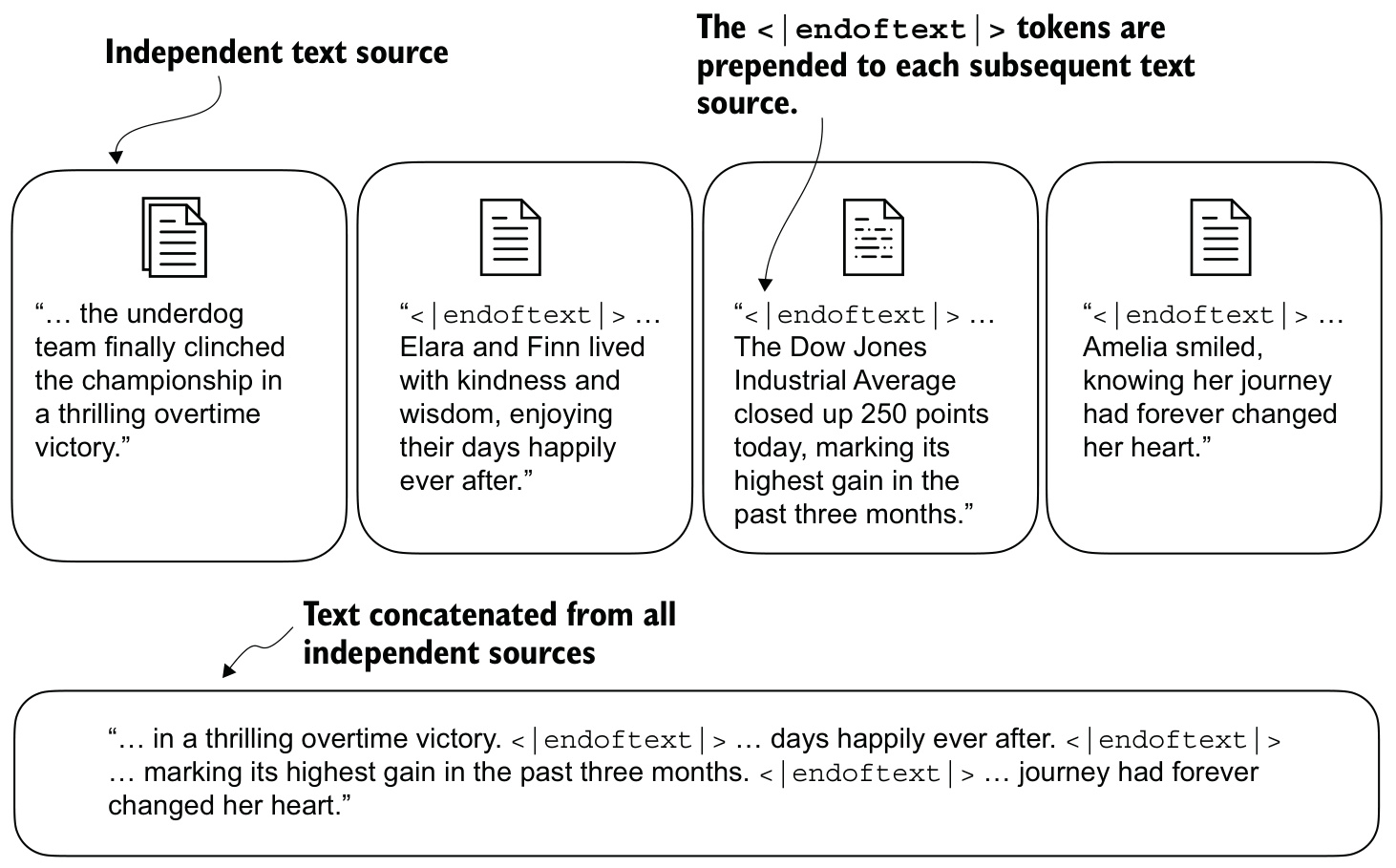
<|endoftext|> tokens placed between independent text sources act as markers signalling the start or end of a particular segment.Both are appended to the sorted unique tokens before the dictionary is built:
all_tokens = sorted(list(set(preprocessed)))
all_tokens.extend(["<|endoftext|>", "<|unk|>"])
vocab = {token:integer for integer,token in enumerate(all_tokens)}

print(len(vocab.items()))
The new vocabulary size is 1,132; it was 1,130. The last five entries confirm where the two tokens landed:
('younger', 1127)
('your', 1128)
('yourself', 1129)
('<|endoftext|>', 1130)
('<|unk|>', 1131)
Listing 2.4 changes one thing in encode: a pass over the token list replaces every out-of-vocabulary token before the integer lookup.
class SimpleTokenizerV2:
    def __init__(self, vocab):
        self.str_to_int = vocab
        self.int_to_str = { i:s for s,i in vocab.items()}

    def encode(self, text):
        preprocessed = re.split(r'([,.:;?_!"()\']|--|\s)', text)
        preprocessed = [
            item.strip() for item in preprocessed if item.strip()
        ]
        preprocessed = [item if item in self.str_to_int
                        else "<|unk|>" for item in preprocessed]

        ids = [self.str_to_int[s] for s in preprocessed]
        return ids

    def decode(self, ids):
        text = " ".join([self.int_to_str[i] for i in ids])

        text = re.sub(r'\s+([,.:;?!"()\'])', r'\1', text)
        return text
Two unrelated sentences joined by the separator:
text1 = "Hello, do you like tea?"
text2 = "In the sunlit terraces of the palace."
text = " <|endoftext|> ".join((text1, text2))
print(text)
Hello, do you like tea? <|endoftext|> In the sunlit terraces of
the palace.Encoding it now succeeds:
[1131, 5, 355, 1126, 628, 975, 10, 1130, 55, 988, 956, 984, 722, 988, 1131, 7]The list contains 1130 for the <|endoftext|> separator and two 1131 tokens for unknown words. Detokenizing shows exactly what was lost:
<|unk|>, do you like tea? <|endoftext|> In the sunlit terraces of
the <|unk|>.
“Hello” and “palace” do not occur in “The Verdict,” and neither survives the round trip.
Depending on the model, researchers use further special tokens:
[BOS](beginning of sequence) marks the start of a text, signifying where a piece of content begins.[EOS](end of sequence) is positioned at the end of a text, and is useful when concatenating multiple unrelated texts. When combining two Wikipedia articles or books,[EOS]indicates where one ends and the next begins.[PAD](padding) extends the shorter texts in a batch up to the length of the longest text, so that all texts in a batch have the same length.
The tokenizer used for GPT models needs none of these. It uses only <|endoftext|>, which is analogous to [EOS] and is also used for padding — when training on batched inputs a mask is applied, so padded tokens are not attended to and the specific token chosen for padding is inconsequential. The GPT tokenizer also uses no <|unk|> token, because it decomposes unfamiliar words into subword units instead.
Learning outcomes
- handle-unknown-tokens Extend a vocabulary with special context tokens to handle unseen words and document boundaries.
Concepts
- special-context-tokens
<|unk|>stands in for a token absent from the vocabulary, and<|endoftext|>marks the boundary between concatenated but unrelated documents - vocabulary-and-token-ids appending two tokens to the sorted unique tokens raises the vocabulary from 1,130 to 1,132 entries and gives each special token an ID of its own
Byte pair encoding
Byte pair encoding (BPE) is the tokenization scheme used to train GPT-2, GPT-3, and the original model used in ChatGPT. Its vocabulary is built by iteratively merging frequent characters into subwords and frequent subwords into words. BPE starts by adding all individual single characters to its vocabulary — “a”, “b”, and so on. In the next stage it merges character combinations that frequently occur together into subwords: “d” and “e” may be merged into the subword “de,” which is common in English words like “define,” “depend,” “made,” and “hidden.” The merges are determined by a frequency cutoff.
The consequence is that the vocabulary is closed under no assumption about the input. If the tokenizer encounters an unfamiliar word, it represents it as a sequence of subword tokens or, in the limit, individual characters.
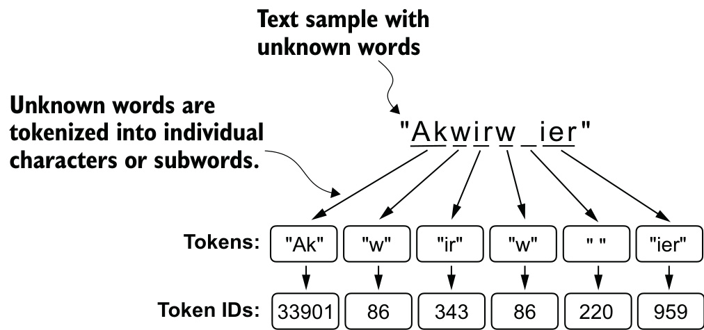
<|unk|>.Implementing BPE is relatively complicated, so the chapter uses OpenAI’s open source library tiktoken, which implements the algorithm on source code written in Rust. The code is based on tiktoken 0.7.0.
tokenizer = tiktoken.get_encoding("gpt2")Its encode method is used much like SimpleTokenizerV2, with one addition — the set of special tokens that are to be recognized rather than split:
text = (
    "Hello, do you like tea? <|endoftext|> In the sunlit terraces"
     "of someunknownPlace."
)
integers = tokenizer.encode(text, allowed_special={"<|endoftext|>"})
print(integers)
[15496, 11, 466, 345, 588, 8887, 30, 220, 50256, 554, 262, 4252, 18250,
8812, 2114, 286, 617, 34680, 27271, 13]strings = tokenizer.decode(integers)
print(strings)Hello, do you like tea? <|endoftext|> In the sunlit terraces of
someunknownPlace.Two observations follow from the IDs and the decoded text.
<|endoftext|>is assigned a relatively large token ID, namely50256. The BPE tokenizer has a total vocabulary size of 50,257, with<|endoftext|>being assigned the largest token ID.someunknownPlaceis encoded and decoded correctly, without any<|unk|>token. It occupies several IDs —617, 34680, 27271— one per subword, and the decode reassembles them exactly.
BPE does not “know” the unfamiliar word. It spells it. The round trip is exact because the concatenation of the subword strings is the original string, not because the tokenizer recognized the word. This is why a word absent from every training corpus still encodes and decodes without loss, while SimpleTokenizerV2 loses it to <|unk|>.
Try the BPE tokenizer on the unknown words “Akwirw ier”, print the individual token IDs, then call decode on each of the resulting integers to reproduce the mapping in figure 2.11. Lastly, call decode on the whole list to check whether it reconstructs the original input.
Figure 2.11 gives the answer: the tokens are "Ak", "w", "ir", "w", " ", "ier", with token IDs 33901, 86, 343, 86, 220, 959.
Learning outcomes
- apply-byte-pair-encoding Use byte pair encoding to tokenize arbitrary text without an out-of-vocabulary failure.
- handle-unknown-tokens Extend a vocabulary with special context tokens to handle unseen words and document boundaries.
Concepts
- byte-pair-encoding a subword vocabulary built by merging frequent adjacent symbols upward from single characters, so any string can be spelled from entries it already holds
- special-context-tokens GPT’s BPE tokenizer carries
<|endoftext|>as its highest ID, 50256, and needs no<|unk|>at all - tokenization subword tokenization replaces word-level splitting, so the unit indexed by the vocabulary is smaller than a word and larger than a character
Data sampling with a sliding window
Training an LLM requires input–target pairs. The target is the word that follows the input block, and every prefix of a sequence is one such pair.
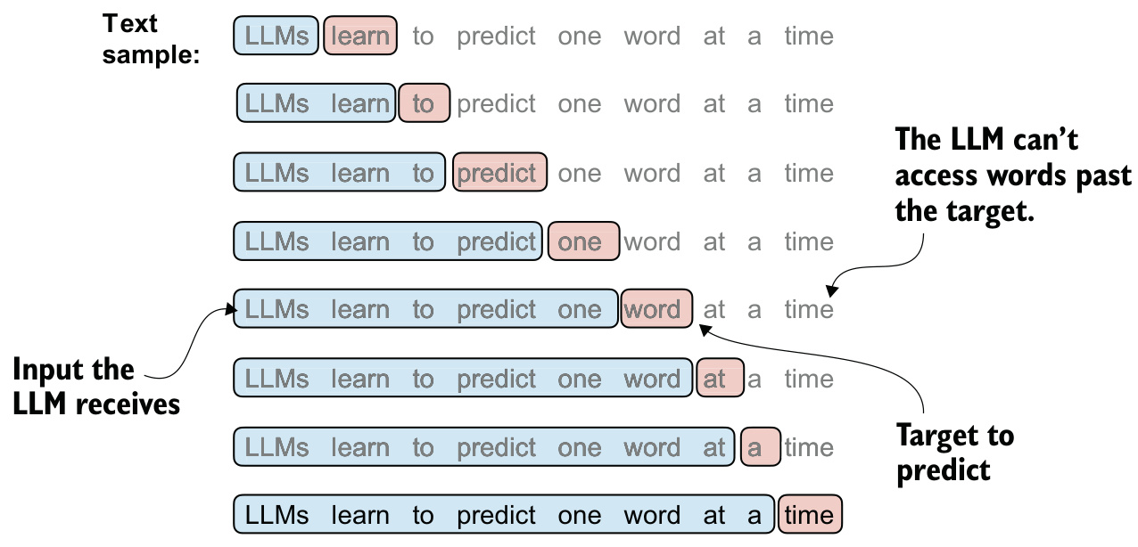
The whole story is tokenized once with the BPE tokenizer:
with open("the-verdict.txt", "r", encoding="utf-8") as f:
    raw_text = f.read()

enc_text = tokenizer.encode(raw_text)
print(len(enc_text))
This returns 5145, the total number of tokens in the training set after applying the BPE tokenizer. The first 50 tokens are removed, which gives a slightly more interesting passage for the illustration:
enc_sample = enc_text[50:]The pair itself is one slice and the same slice advanced by one:
context_size = 4
x = enc_sample[:context_size]
y = enc_sample[1:context_size+1]
print(f"x: {x}")
print(f"y:      {y}")
x: [290, 4920, 2241, 287]
y: [4920, 2241, 287, 257]Reading the pair position by position gives four prediction tasks out of one window of four tokens:
for i in range(1, context_size+1):
    context = enc_sample[:i]
    desired = enc_sample[i]
    print(context, "---->", desired)
[290] ----> 4920
[290, 4920] ----> 2241
[290, 4920, 2241] ----> 287
[290, 4920, 2241, 287] ----> 257Decoding both sides shows the same four tasks as text:
 and ---->  established
 and established ---->  himself
 and established himself ---->  in
 and established himself in ---->  a
The dataset and the loader
Listing 2.5 stores every window as a pair of tensors. The loop is the sliding window: it starts at 0, advances by stride, and stops max_length tokens before the end of the stream so that the target chunk is never short.
import torch
from torch.utils.data import Dataset, DataLoader

class GPTDatasetV1(Dataset):
    def __init__(self, txt, tokenizer, max_length, stride):
        self.input_ids = []
        self.target_ids = []

        token_ids = tokenizer.encode(txt)

        for i in range(0, len(token_ids) - max_length, stride):
            input_chunk = token_ids[i:i + max_length]
            target_chunk = token_ids[i + 1: i + max_length + 1]
            self.input_ids.append(torch.tensor(input_chunk))
            self.target_ids.append(torch.tensor(target_chunk))

    def __len__(self):
        return len(self.input_ids)

    def __getitem__(self, idx):
        return self.input_ids[idx], self.target_ids[idx]
Listing 2.6 wraps the dataset in a PyTorch DataLoader:
def create_dataloader_v1(txt, batch_size=4, max_length=256,
                         stride=128, shuffle=True, drop_last=True,
                         num_workers=0):
    tokenizer = tiktoken.get_encoding("gpt2")
    dataset = GPTDatasetV1(txt, tokenizer, max_length, stride)
    dataloader = DataLoader(
        dataset,
        batch_size=batch_size,
        shuffle=shuffle,
        drop_last=drop_last,
        num_workers=num_workers
    )

    return dataloader
drop_last=True drops the last batch if it is shorter than the specified batch_size, which prevents loss spikes during training. num_workers is the number of CPU processes used for preprocessing.
Choosing the stride
With batch_size=1, max_length=4 and stride=1, the first two batches are:
[tensor([[  40,  367, 2885, 1464]]), tensor([[ 367, 2885, 1464, 1807]])]
[tensor([[ 367, 2885, 1464, 1807]]), tensor([[2885, 1464, 1807, 3619]])]
The second batch’s token IDs are shifted by one position relative to the first — the second ID in the first batch’s input, 367, is the first ID of the second batch’s input. The stride dictates the number of positions the inputs shift across batches.
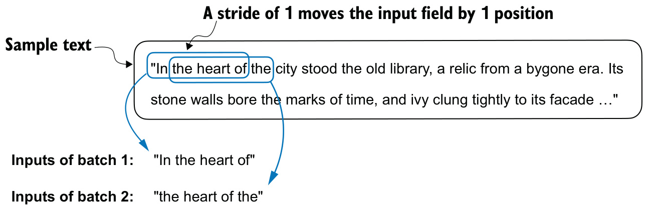
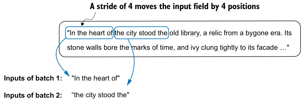
With batch_size=8, max_length=4 and stride=4, each of the eight rows is a separate context and the batches do not overlap:
Inputs:
 tensor([[   40,   367,  2885,  1464],
        [ 1807,  3619,   402,   271],
        [10899,  2138,   257,  7026],
        [15632,   438,  2016,   257],
        [  922,  5891,  1576,   438],
        [  568,   340,   373,   645],
        [ 1049,  5975,   284,   502],
        [  284,  3285,   326,    11]])

Targets:
 tensor([[  367,  2885,  1464,  1807],
        [ 3619,   402,   271, 10899],
        [ 2138,   257,  7026, 15632],
        [  438,  2016,   257,   922],
        [ 5891,  1576,   438,   568],
        [  340,   373,   645,  1049],
        [ 5975,   284,   502,   284],
        [ 3285,   326,    11,   287]])
Setting the stride to 4 utilizes the dataset fully — not a single word is skipped — and avoids overlap between the batches, since more overlap could lead to increased overfitting. An input size of 4 is chosen only for simplicity; it is common to train LLMs with input sizes of at least 256. Small batch sizes require less memory during training but lead to more noisy model updates, so batch size is a hyperparameter to experiment with.
Run the data loader with max_length=2 and stride=2, and with max_length=8 and stride=2, and observe how the batches are formed and how far the window shifts.
Learning outcomes
- build-sliding-window-dataloader Generate input–target pairs for next-token prediction with a sliding window, and load them in batches.
Concepts
- sliding-window-data-sampling a window of
max_lengthtokens advancing bystrideyields an input chunk and a target chunk that is the same chunk advanced by one position - vocabulary-and-token-ids the loader operates on token IDs directly, because the BPE
encodemethod performs tokenization and integer conversion as a single step
The token embedding layer
The DataLoader yields integers. The transformer requires vectors. Converting the token IDs into embedding vectors is the last step in preparing the input text.
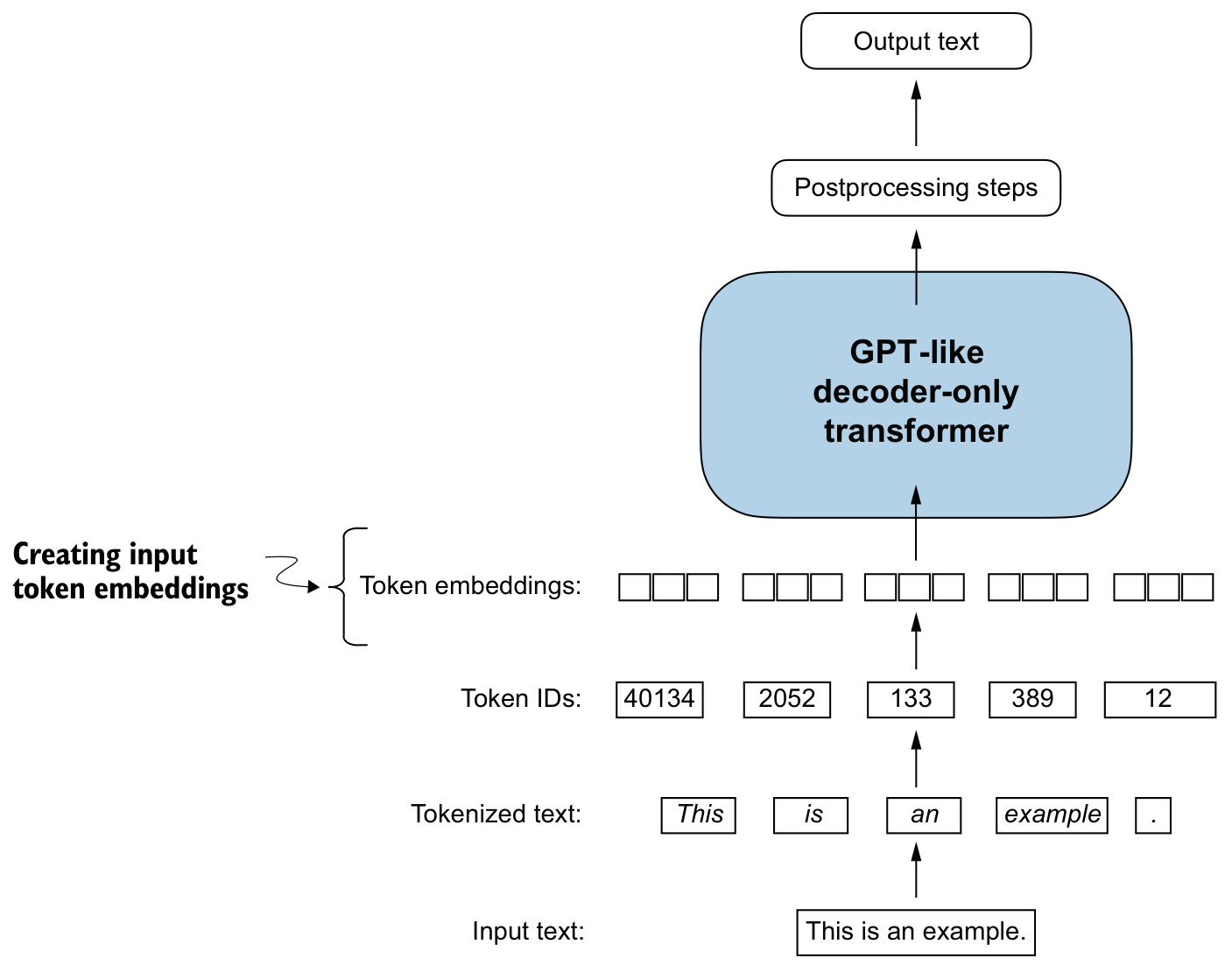
The embedding weights are initialized with random values, which serve as the starting point for the model’s learning process; they are optimized as part of LLM training itself. A continuous vector representation is necessary because GPT-like LLMs are deep neural networks trained with the backpropagation algorithm.
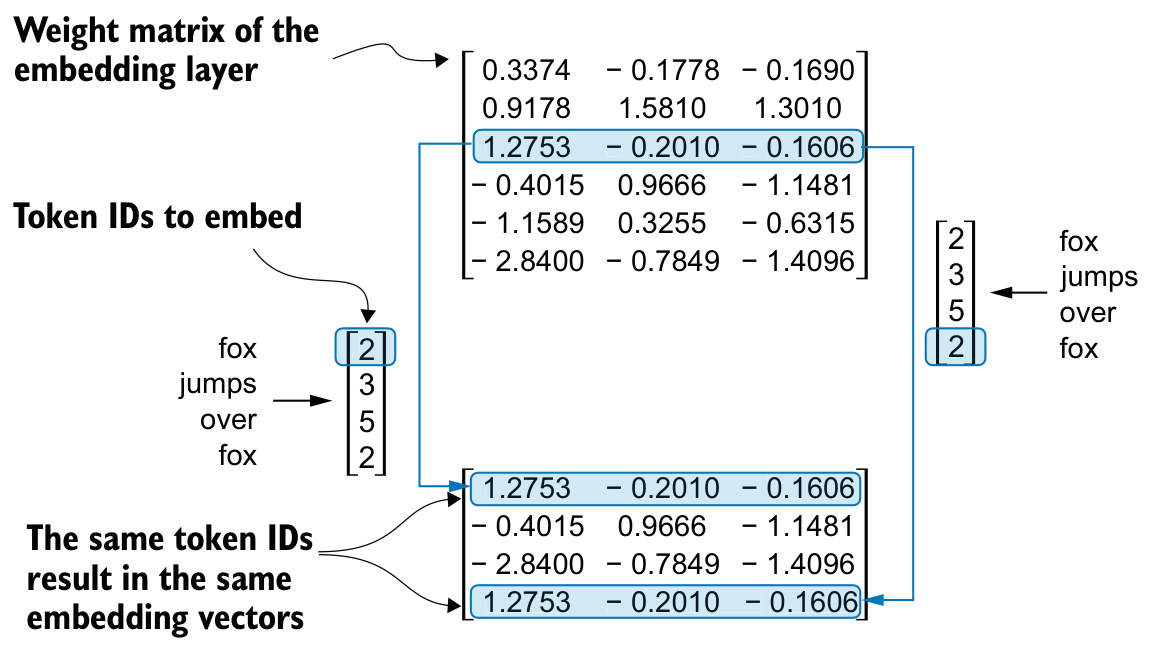
Take four input tokens with IDs 2, 3, 5 and 1, a vocabulary of only 6 words, and embeddings of size 3:
input_ids = torch.tensor([2, 3, 5, 1])vocab_size = 6
output_dim = 3torch.manual_seed(123)
embedding_layer = torch.nn.Embedding(vocab_size, output_dim)
print(embedding_layer.weight)Parameter containing:
tensor([[ 0.3374, -0.1778, -0.1690],
[ 0.9178, 1.5810, 1.3010],
[ 1.2753, -0.2010, -0.1606],
[-0.4015, 0.9666, -1.1481],
[-1.1589, 0.3255, -0.6315],
[-2.8400, -0.7849, -1.4096]], requires_grad=True)The weight matrix has six rows and three columns: one row for each of the six possible tokens in the vocabulary, and one column for each of the three embedding dimensions. Applying the layer to a single ID:
print(embedding_layer(torch.tensor([3])))tensor([[-0.4015, 0.9666, -1.1481]], grad_fn=<EmbeddingBackward0>)The returned vector is identical to the fourth row of the weight matrix, because Python starts with a zero index and so row index 3 is the fourth row. The embedding layer is a lookup operation that retrieves rows from the weight matrix via a token ID. Applied to all four IDs it returns a \(4 \times 3\) matrix:
print(embedding_layer(input_ids))tensor([[ 1.2753, -0.2010, -0.1606],
[-0.4015, 0.9666, -1.1481],
[-2.8400, -0.7849, -1.4096],
[ 0.9178, 1.5810, 1.3010]], grad_fn=<EmbeddingBackward0>)The embedding layer approach is a more efficient way of implementing one-hot encoding followed by matrix multiplication in a fully connected layer. Because the layer is just a more efficient implementation equivalent to the one-hot encoding and matrix-multiplication approach, it can be seen as a neural network layer that can be optimized via backpropagation. The gradient is what makes the two forms equivalent in training, not only in the forward pass.
With a vocabulary of 50,257 and an embedding size of 256, the one-hot form would materialise a \(B \times L \times 50257\) matrix before the multiply. The lookup form never constructs it.
Learning outcomes
- create-token-embeddings Turn token IDs into vectors with an
nn.Embeddinglayer, and explain what that layer really is.
Concepts
- word-embeddings the embedding layer is a learnable weight matrix of shape (vocabulary size \(\times\) embedding dimension) whose rows are the token vectors
- vocabulary-and-token-ids a token ID is used as a row index into that weight matrix, so the vocabulary fixes the number of rows the layer must hold
Encoding word positions
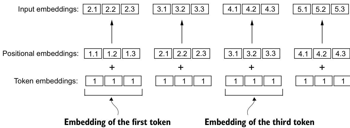
The embedding of a token ID is deterministic and position-independent, which is good for reproducibility. It is also a shortcoming: the same token ID always gets mapped to the same vector representation, regardless of where it is positioned in the input sequence, and the self-attention mechanism of an LLM is itself position-agnostic.
Two broad categories of position-aware embedding exist.
Absolute positional embeddings are directly associated with specific positions in a sequence. For each position in the input sequence, a unique embedding is added to the token’s embedding to convey its exact location — the first token has a specific positional embedding, the second another distinct embedding, and so on.
OpenAI’s GPT models use absolute positional embeddings that are optimized during the training process, rather than being fixed or predefined like the positional encodings in the original transformer model.
Relative positional embeddings place the emphasis on the relative position, or distance, between tokens. The model learns the relationships in terms of “how far apart” rather than “at which exact position.”
The advantage is that the model can generalize better to sequences of varying lengths, even if it has not seen such lengths during training.
Both types aim to augment the capacity of an LLM to understand the order and relationships between tokens. The choice between them depends on the application and the nature of the data.
Assembling the input embedding
The working configuration uses an embedding size of 256 — smaller than GPT-3’s 12,288, but reasonable for experimentation — and the 50,257-token BPE vocabulary:
vocab_size = 50257
output_dim = 256
token_embedding_layer = torch.nn.Embedding(vocab_size, output_dim)
A batch of eight samples with four tokens each is drawn from the loader with the stride set equal to max_length:
max_length = 4
dataloader = create_dataloader_v1(
     raw_text, batch_size=8, max_length=max_length,
    stride=max_length, shuffle=False
)
data_iter = iter(dataloader)
inputs, targets = next(data_iter)
print("Token IDs:\n", inputs)
print("\nInputs shape:\n", inputs.shape)
The token ID tensor is torch.Size([8, 4]) — eight text samples with four tokens each. Embedding it gives one 256-dimensional vector per token:
token_embeddings = token_embedding_layer(inputs)
print(token_embeddings.shape)
torch.Size([8, 4, 256])The positional layer has the same embedding dimension, but is indexed by position rather than by token:
context_length = max_length
pos_embedding_layer = torch.nn.Embedding(context_length, output_dim)
pos_embeddings = pos_embedding_layer(torch.arange(context_length))
print(pos_embeddings.shape)
torch.Size([4, 256])The input to pos_embeddings is usually the placeholder vector torch.arange(context_length), which contains the sequence of numbers 0, 1, …, up to the maximum input length minus one. context_length is the variable representing the supported input size of the LLM; it is chosen here to be similar to the maximum length of the input text. In practice input text can be longer than the supported context length, in which case the text has to be truncated.
The two tensors are then added. PyTorch adds the \(4 \times 256\)-dimensional pos_embeddings tensor to each \(4 \times 256\)-dimensional token embedding tensor in each of the eight batches:
input_embeddings = token_embeddings + pos_embeddings
print(input_embeddings.shape)
torch.Size([8, 4, 256])The positional tensor has three axes fewer than one might expect — it is \(4 \times 256\), not \(8 \times 4 \times 256\). Broadcasting supplies the missing batch axis by applying the same four positional vectors to every example in the batch. That is the intended behaviour: position 0 means the same thing in every sample, so the positional vector for it must be shared, not per-example.
Learning outcomes
- add-positional-embeddings Add absolute positional embeddings to token embeddings to produce the model’s final input.
Concepts
- positional-embeddings a second embedding layer indexed by position, of the same dimension as the token embeddings, is added element-wise so that identical tokens at different positions differ
- word-embeddings the sum of the token embedding and the positional embedding is the input embedding, and both summands are learned during training
What the pipeline produces
Key ideas
LLMs require textual data to be converted into numerical vectors, known as embeddings, since they cannot process raw text.
Embeddings transform discrete data, like words or images, into continuous vector spaces, making them compatible with neural network operations.
As the first step, raw text is broken into tokens, which can be words or characters, and the tokens are then converted into integer representations, termed token IDs.
The split is an explicit set of choices — which punctuation is its own token, whether whitespace survives, whether case is preserved — and each one is recoverable from the regular expression.
Special tokens, such as
<|unk|>and<|endoftext|>, can be added to enhance the model’s understanding and handle various contexts, such as unknown words or marking the boundary between unrelated texts.A closed vocabulary raises a
KeyErroron any word it has not seen;<|unk|>converts that failure into a loss of information.The byte pair encoding tokenizer used for LLMs like GPT-2 and GPT-3 can efficiently handle unknown words by breaking them down into subword units or individual characters.
This is why the GPT tokenizer needs no
<|unk|>token at all, and why its round trip onsomeunknownPlaceis exact.A sliding window approach on tokenized data generates input–target pairs for LLM training.
A stride equal to
max_lengthuses every token exactly once and produces no overlap between batches, since more overlap could lead to increased overfitting.Embedding layers in PyTorch function as a lookup operation, retrieving vectors corresponding to token IDs.
The lookup is a more efficient implementation of one-hot encoding followed by a matrix multiplication, and remains a layer that can be optimized by backpropagation.
While token embeddings provide consistent vector representations for each token, they lack a sense of the token’s position in a sequence. OpenAI’s GPT models use absolute positional embeddings, which are added to the token embedding vectors and are optimized during model training.
Without them, self-attention receives its input as an unordered set, and the tensor for “a b” would be a permutation of the tensor for “b a”.
The finished pipeline hands over a tensor of shape (batch \(\times\) context length \(\times\) embedding dimension). The next unit, 3 Coding attention mechanisms, builds the layer that consumes it: attention scores from dot products of query and key projections, normalization by softmax after scaling by \(\sqrt{d_k}\), a weighted sum of value vectors, then causal masking that sets scores above the diagonal to \(-\infty\) so no position can attend to the future, and finally an efficient batched multi-head implementation.
References
- Building a Large Language Model (from scratch), Sebastian Raschka, 2024, Manning Books — Link — Page 39-71