2 Working with text data

Language Models · v1.0.0

2026-08-25 14:45:28

Where we are

From string to matrix

A transformer accepts a matrix of numbers. Your corpus is a string. This unit is the whole distance between the two.

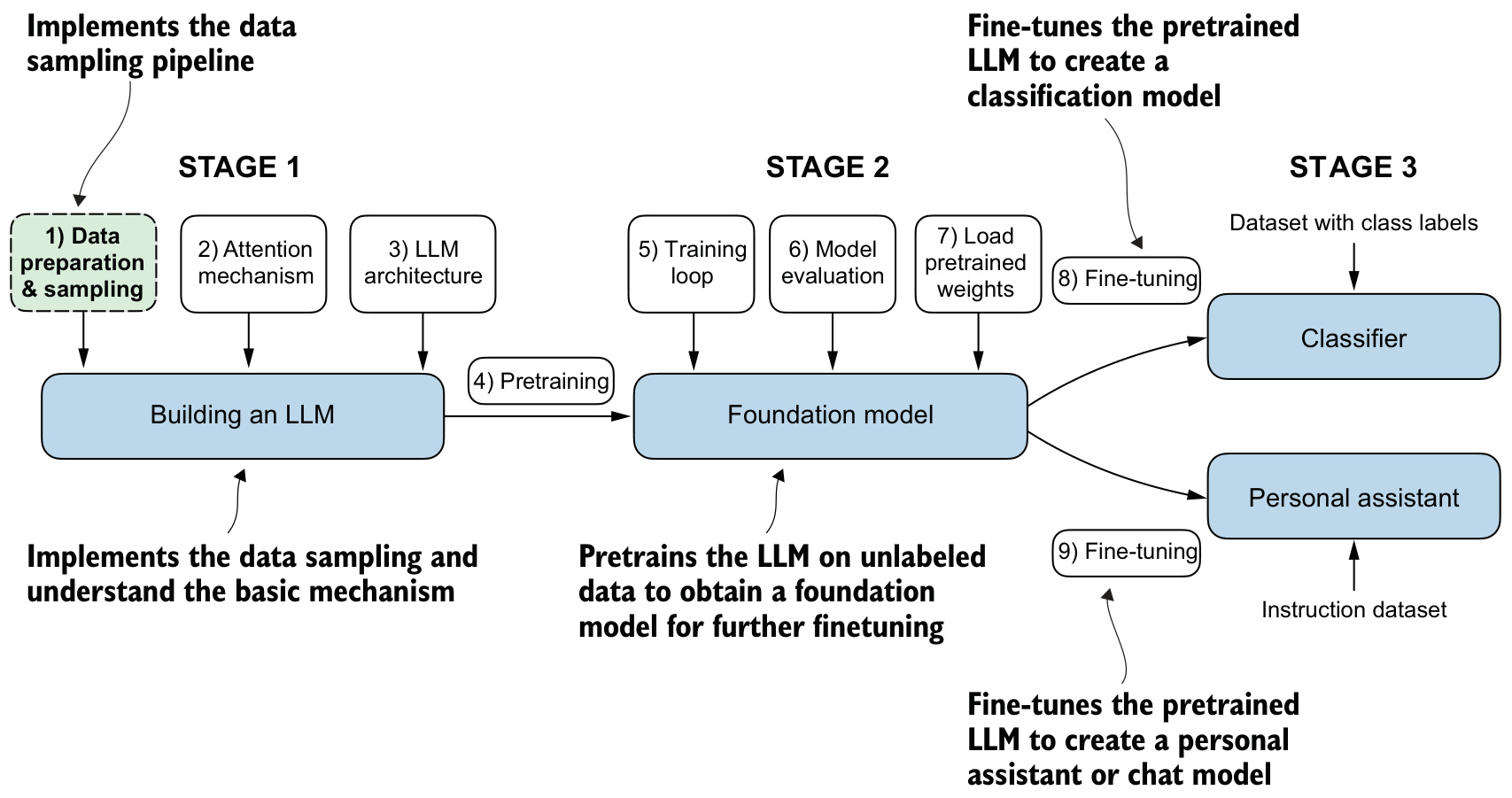
This unit is step 1 of stage 1: the data sampling pipeline.

Previous unit established what an LLM is and the three-stage roadmap. This unit begins stage 1, step 1: data preparation and sampling.

The pipeline

• Tokenize the raw text into words, punctuation and sub-word units
• Map each token to an integer token ID through a vocabulary
• Look up an embedding vector for each ID
• Add positional information so the model knows where each token sat

Along the way: what does the tokenizer do with an unseen word, and how do we cut one token stream into training examples?

Source: Raschka, Build a Large Language Model (from scratch), chapter 2. These notes give concepts and terse pseudocode, not working implementations — read the source for the full listings.

Why text has to become vectors

Embeddings, formally

Neural networks operate on continuous values; text is categorical. An embedding maps discrete tokens into a continuous vector space.

\[E : V \to \mathbb{R}^{d}\]

Since \(V\) is finite, \(E\) is fully described by a matrix \(\mathbf{W} \in \mathbb{R}^{|V| \times d}\), one row per token.

This is the fact we return to when we build the embedding layer. An embedding model designed for text would not suit audio or video — different data formats need distinct embedding models.

Word2Vec and the shape of the space

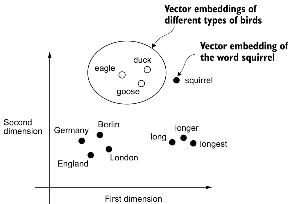
2D word embeddings: similar concepts cluster together.

• Predicts a word’s context, or the reverse
• Words in similar contexts land close together
• One of the earliest popular embedding algorithms

Standalone versus in-model embeddings

LLMs typically produce their own embeddings, as part of the input layer, updated during training — rather than reusing a pretrained model like Word2Vec.

• Smallest GPT-2 models: 768 dimensions
• Largest GPT-3 model: 12,288 dimensions

Higher dimensionality captures more nuance, at the cost of computational efficiency.

Tokenizing text

Splitting text into tokens

Tokenization splits input text into individual tokens — words or special characters, including punctuation.

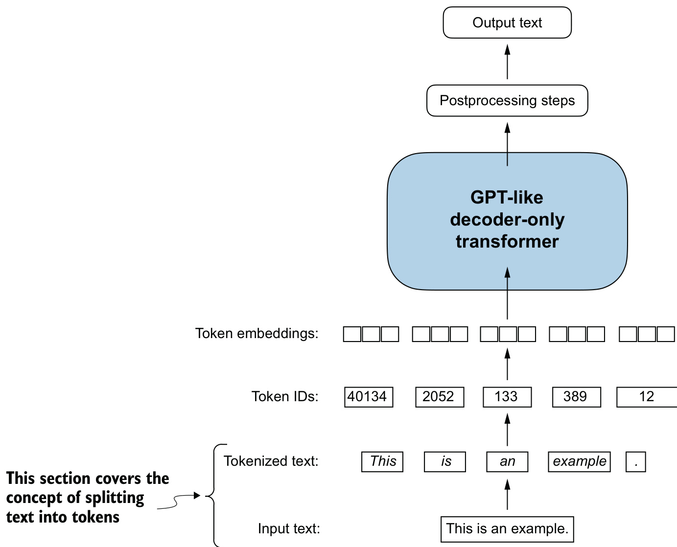
Splitting text into individual tokens.

Working corpus: “The Verdict” by Edith Wharton, public domain, 20,479 characters — small enough that every intermediate result stays inspectable by eye.

Building the split, one decision at a time

A tokenizer is a function \(T : \Sigma^{*} \to V^{*}\). The chapter arrives at its rule in three steps.

1. Split on whitespace — punctuation stays glued to words
2. Split on whitespace, commas and periods — filter empty strings
3. Extend to the remaining punctuation: ? : ; " ( ) --

The rule, as pseudocode

DELIMITERS = r'([,.:;?_!"()\']|--|\s)'

def tokenize(text):
    pieces = split_on(DELIMITERS, text)
    return [p for p in pieces if not_blank(p)]

• Case is preserved — helps distinguish proper nouns, sentence structure
• Punctuation is a token — keeps the vocabulary small ("world" and "world." are one entry) while remaining a signal

Applied to the whole short story, this rule yields 4,690 tokens. Raschka §2.2 develops the expression line by line and prints output at each stage.

From tokens to token IDs

Building the vocabulary

A vocabulary maps each unique token to a unique integer, built by tokenizing the corpus, taking the set, sorting and numbering.

\[V = \operatorname{sorted}(\operatorname{set}(T(\text{corpus}))), \qquad \mathrm{id}(v_i) = i\]

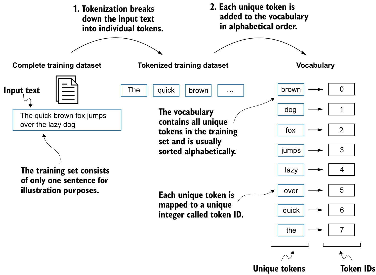
A vocabulary built by sorting unique tokens and numbering them.

“The Verdict” gives a vocabulary of 1,130 entries — far fewer than 4,690 tokens, because most words recur. Sorting only makes assignment deterministic and inspectable, not required for correctness.

A tokenizer class

Since \(\mathrm{id}\) is a bijection between \(V\) and \(\{0, \dots, |V|-1\}\), one vocabulary supplies both directions.

class SimpleTokenizer:
    def __init__(self, vocab):
        self.str_to_int = vocab
        self.int_to_str = invert(vocab)

    def encode(self, text) -> list[int]:
        return [self.str_to_int[t] for t in tokenize(text)]

    def decode(self, ids) -> str:
        text = join_with_space(self.int_to_str[i] for i in ids)
        return reattach_punctuation(text)

The detokenization step in decode matters: joining tokens with a single space would leave a space before every comma and period, so punctuation must be re-attached. encode and decode are inverses only up to that whitespace convention.

The failure mode

Apply this tokenizer outside the training set and it fails outright.

Encoding "Hello, do you like tea?" raises a lookup error — Hello never occurs in “The Verdict”.

This is not a bug. It is a property of a closed vocabulary built from one small corpus.

Special context tokens

Two new tokens

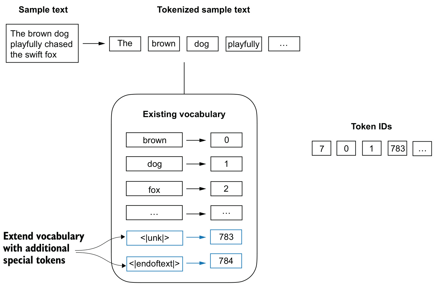
Special tokens <|unk|> and <|endoftext|> added to the vocabulary.

• <|unk|> — stands in for a word outside the vocabulary, so encode returns an ID instead of raising
• <|endoftext|> — inserted before each document that follows a previous, unrelated text source

Both appended after observed tokens, taking the two highest IDs. Vocabulary grows from 1,130 to 1,132 entries: endoftext at 1130, unk at 1131. Information is lost when unk is used — every unknown word decodes to the same string.

A tokenizer that survives

The repair is one line in encode: substitute before looking up, so no lookup can miss.

def encode(self, text):
    tokens = tokenize(text)
    tokens = [t if known(t) else "<|unk|>" for t in tokens]
    return [self.str_to_int[t] for t in tokens]

decode is unchanged — the unknown token round-trips as the literal string <|unk|>.

Other special tokens

[BOS], [EOS], [PAD] mark sequence start, sequence end, and batch padding.

GPT models use none of these — only <|endoftext|>, which doubles as end-marker and padding token, and no <|unk|>, because GPT uses byte pair encoding instead.

Byte pair encoding

Removing the closed-vocabulary failure

Byte pair encoding (BPE) is the tokenization scheme used to train GPT-2, GPT-3 and the original ChatGPT model.

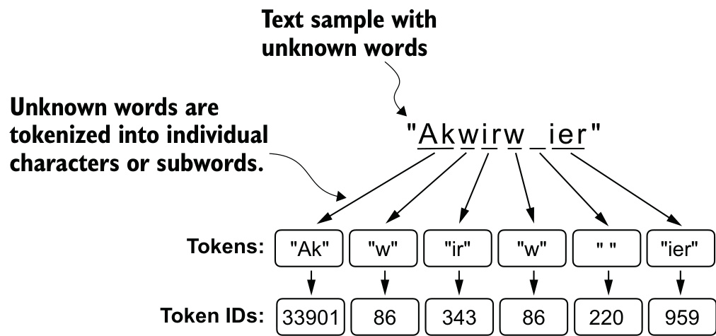
Rather than a fixed token set, BPE admits sub-word units, so any string can be spelled from pieces the vocabulary already holds.

In practice, one uses an existing implementation — tiktoken, exposing the same encode/decode interface.

Two properties that matter downstream

• <|endoftext|> is assigned token ID 50256 — the vocabulary size is 50,257
• An invented word like someunknownPlace encodes and decodes correctly, with no <|unk|> token

Unknown words broken into sub-words and characters.

How the vocabulary is built

• Start with all individual characters
• Merge frequent character combinations into sub-words ("d" + "e" → "de")
• Repeat, guided by a frequency cutoff

def train_bpe(corpus, num_merges):
    vocab = set(all_characters(corpus))
    for _ in range(num_merges):
        a, b = most_frequent_adjacent_pair(corpus, vocab)
        vocab.add(a + b)
        corpus = replace_pair(corpus, a, b)
    return vocab

Because every character is in the vocabulary from the start, encoding can always terminate — in the worst case a word is spelled character by character. That guarantee is what makes an unseen word processable at all.

Data sampling with a sliding window

Generating input-target pairs

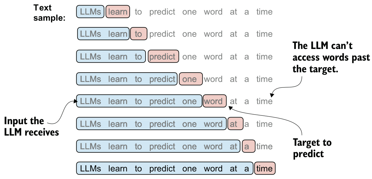
Input blocks predict the word following each block.

BPE-tokenizing “The Verdict” gives a single stream of 5,145 token IDs. The sampling problem: how to cut it into supervised examples.

The window and the shift

Fix a context size \(n\). For a window at position \(i\):

\[\mathbf{x}^{(i)} = (t_i, \dots, t_{i+n-1}), \qquad \mathbf{y}^{(i)} = (t_{i+1}, \dots, t_{i+n})\]

The target at every position is the token that actually followed it — one window of length \(n\) carries \(n\) prediction tasks.

predict t_{i+1} from t_i; predict t_{i+2} from t_i, t_{i+1}; and so on up to the full context. Example: “and” -> “established”, “and established” -> “himself”, “and established himself” -> “in”.

The dataset and the loader

class GPTDataset:
    def __init__(self, text, tokenizer, max_length, stride):
        ids = tokenizer.encode(text)
        self.pairs = [
            (ids[i : i+max_length], ids[i+1 : i+max_length+1])
            for i in range(0, len(ids) - max_length, stride)
        ]

• max_length — the context size \(n\)
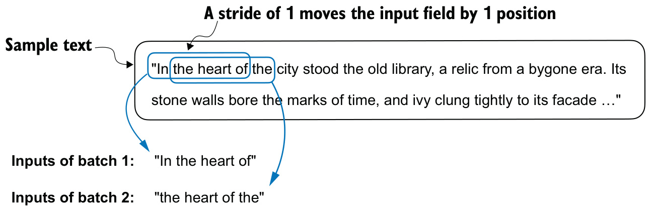
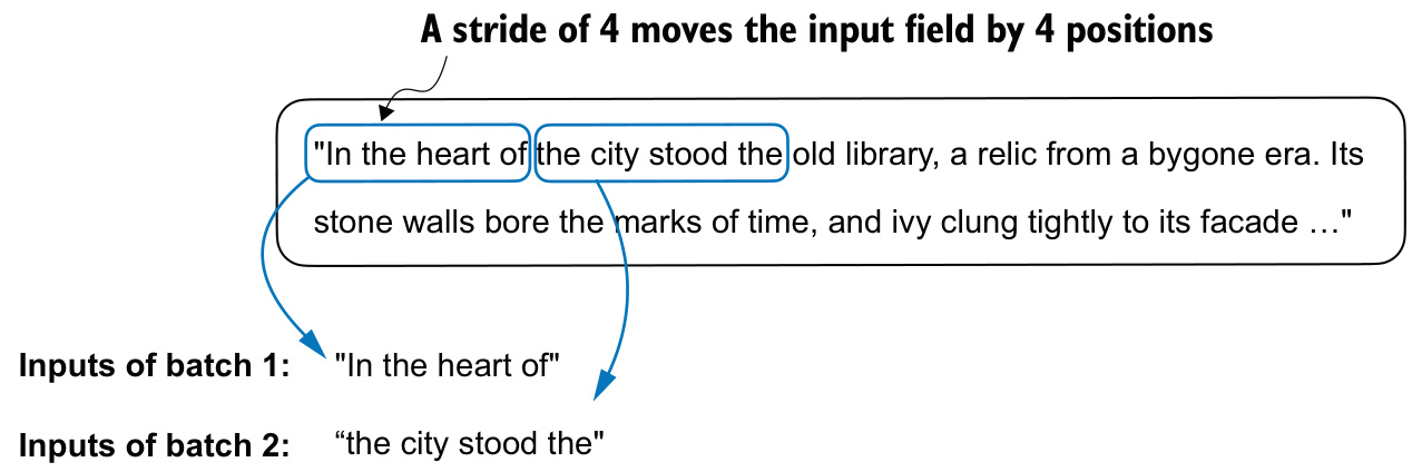
• stride — how far the window advances between examples

A standard batching loader groups pairs into tensors of shape (batch size x context length). Dropping a final short batch keeps every batch the same shape, which prevents loss spikes during training.

Choosing the stride \(^1/_2\)

Stride of 1: maximal overlap.

Stride equal to window size: no overlap.

Choosing the stride \(^2/_2\)

• stride = 1 — each token appears in up to \(n\) examples: maximally large, maximally redundant
• stride = max_length — windows tile without overlap: each token used once per epoch

The chapter settles on the non-overlapping choice to use the dataset fully without skipping words, since more overlap risks overfitting.

Batch size is a separate tradeoff: small batches need less memory but give noisier updates — a hyperparameter to experiment with.

The token embedding layer

From token ID to vector

An embedding is a weight matrix \(\mathbf{W} \in \mathbb{R}^{|V| \times d}\). Embedding a token ID selects its row:

\[E(t) = \mathbf{W}_{t,:}\]

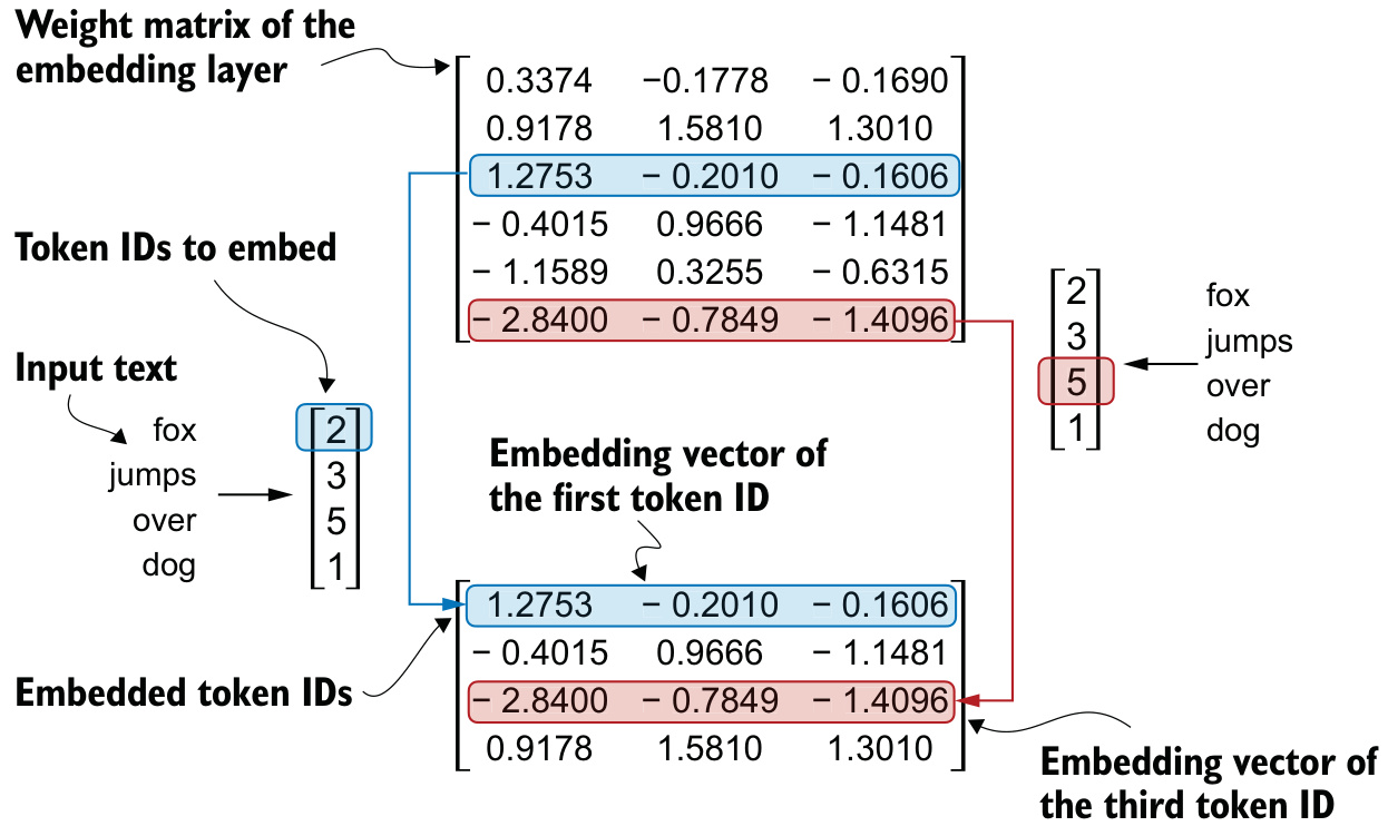
The embedding layer retrieves a row per token ID.

Applied to a sequence of n IDs, returns an n x d matrix; applied to a batch of B sequences, a B x n x d tensor. Weights start random and are optimised as part of LLM training.

Why a lookup, not one-hot

The embedding layer is a more efficient implementation of one-hot encoding followed by a fully connected layer.

\[\mathbf{e}_t^{\top} \mathbf{W} = \mathbf{W}_{t,:}\]

Same map, different cost — and because it is equivalent to a linear layer, it can be optimized via backpropagation.

Encoding word positions

The missing piece

The embedding layer maps the same token ID to the same vector, regardless of position.

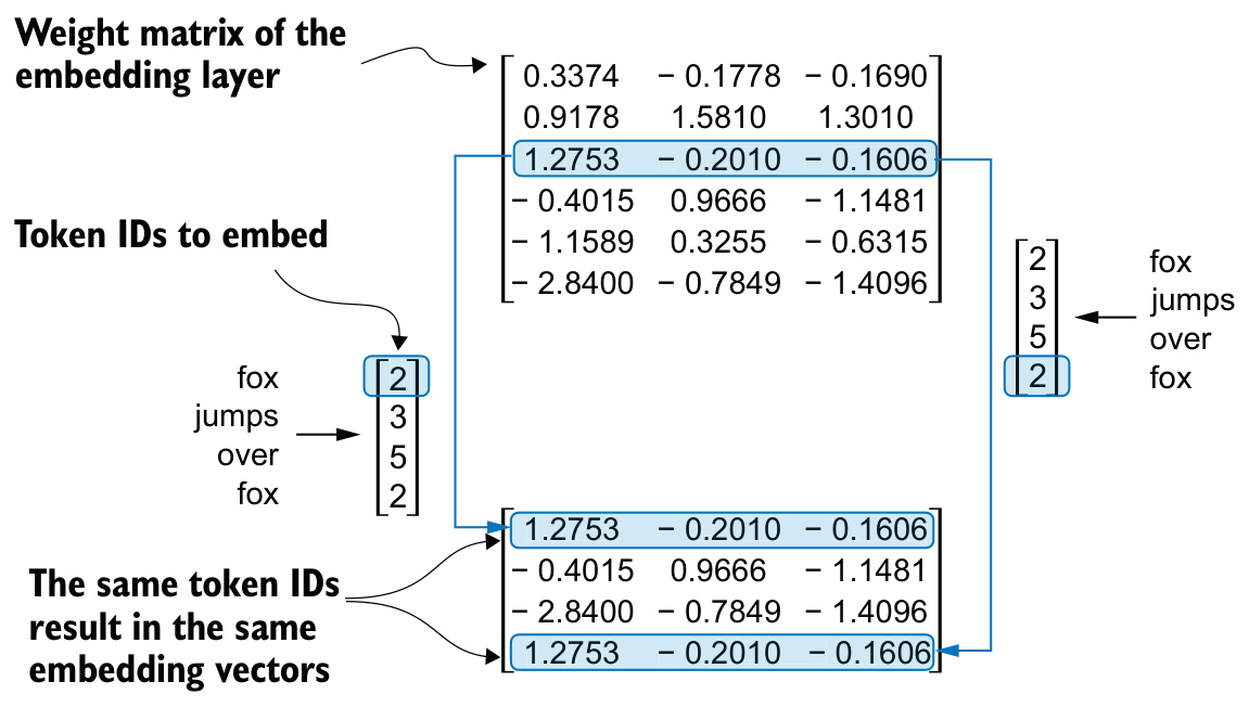
Token ID 5 gives the same vector in the first or fourth position.

Self-attention itself has no notion of order — position must be injected separately.

Two kinds of positional embedding

• Absolute — a unique embedding added per position, conveying exact location
• Relative — encodes distance between tokens, generalizes better across sequence lengths

OpenAI’s GPT models use absolute positional embeddings, optimized during training. That is what we implement.

Assembling the input embedding

table	rows	indexed by
token embedding	\(\lvert V \rvert\) = 50,257	token ID
positional embedding	context length \(n\)	position \(0,\dots,n-1\)

\[\mathbf{Z}_{b,i,:} = E_{\text{tok}}(t_{b,i}) + E_{\text{pos}}(i)\]

token_emb = Embedding(vocab_size, d)      # 50257 x d
pos_emb   = Embedding(context_length, d)  #     n x d
Z = token_emb(batch) + pos_emb(arange(context_length))

The addition broadcasts: the same n x d positional matrix adds to every example in the batch, since position i means the same thing in every sequence. With batch 8, context 4, d=256: token IDs of shape 8x4 become an embedding of shape 8x4x256.

What we have built

The pipeline, complete

• Text becomes tokens, tokens become token IDs, via a vocabulary that is a bijection
• Special tokens (<|unk|>, <|endoftext|>) carry information about the text, not part of it
• BPE removes the closed-vocabulary failure by admitting sub-words
• A sliding window turns one token stream into input-target pairs
• Embedding layers are a lookup table, optimized like any other layer
• Positional embeddings restore the order information self-attention lacks

Where next

The pipeline hands over a tensor of shape (batch size \(\times\) context length \(\times\) embedding dimension).

Next: 3 Coding attention mechanisms. Self-attention, from a simplified form through trainable weights, causal masking, dropout, and a batched multi-head formulation.