Lecture notes — 3 Coding attention mechanisms
ver. 1.2.0, 3_coding_attention_mechanisms
← 3 Coding attention mechanisms
ver. 1.2.0 · 2026-09-02 16:27:30
Where this fits
The previous unit, 2 Working with text data, produced the tensor an LLM actually consumes: token IDs from byte pair encoding, mapped through torch.nn.Embedding to dense vectors, with learnable absolute positional embeddings added element-wise. Its output has shape (batch size, sequence length, embedding dimension).
That tensor is static. A token embedding is the same vector wherever the token occurs, and the positional embedding added to it depends only on the slot, not on the neighbours. Attention is the layer that makes a token’s representation depend on the other tokens present. Each position produces a context vector — an enriched embedding built from every position in the sequence — and the chapter builds that computation in four passes: a simplified mechanism with no parameters, one with trainable projections, one that masks the future, and one that runs several mechanisms in parallel.
Source for this unit: Building a Large Language Model (from scratch), Sebastian Raschka, 2024, Manning Books, chapter 3, pages 50–91.
Learning outcomes
explain-rnn-bottleneck— Explain the information bottleneck of RNN encoder-decoder models and how attention removes it.compute-context-vector— Compute a context vector for one query token with the three-step attention pipeline and no trainable weights.vectorize-over-all-tokens— Vectorize the attention computation so every token gets its context vector in one matrix operation.implement-trainable-attention— Implement self-attention with trainable query, key and value projection matrices and scaled dot products.package-attention-module— Package self-attention as a compactnn.Module, usingnn.Linearrather than rawnn.Parameter.apply-causal-mask— Apply a causal mask so that no token can attend to a token that follows it.apply-attention-dropout— Regularize attention with dropout, and account for the rescaling it applies.handle-batched-inputs— Write an attention module that handles batched inputs of shape (batch, tokens, dimension).implement-multi-head-attention— Implement multi-head causal attention, first by stacking heads and then by splitting one large projection.
Concepts introduced
- Self-attention — a mechanism that relates different positions within a single input sequence, mapping the sequence to enriched representations called context vectors.
- Dot-product attention score — the dot product of two vectors, used as a measure of alignment; a higher value means the two vectors are more closely aligned, and the resulting scalar is written \(\omega\).
- Query, key and value projections — trainable matrices \(W_q\), \(W_k\) and \(W_v\) that map each input embedding into three roles borrowed from database terminology: the item being looked up, the index it is matched against, and the content retrieved.
- Scaled dot-product attention — self-attention in which the scores are divided by the square root of the key embedding dimension before the softmax.
- Causal attention — masked attention, in which a token’s attention weights over positions after it are forced to zero.
- Attention weight dropout — dropout applied to the normalized attention weights during training, with the survivors rescaled.
- Multi-head attention — several attention mechanisms with separate weight matrices run in parallel, their context vectors concatenated.
The problem with modeling long sequences
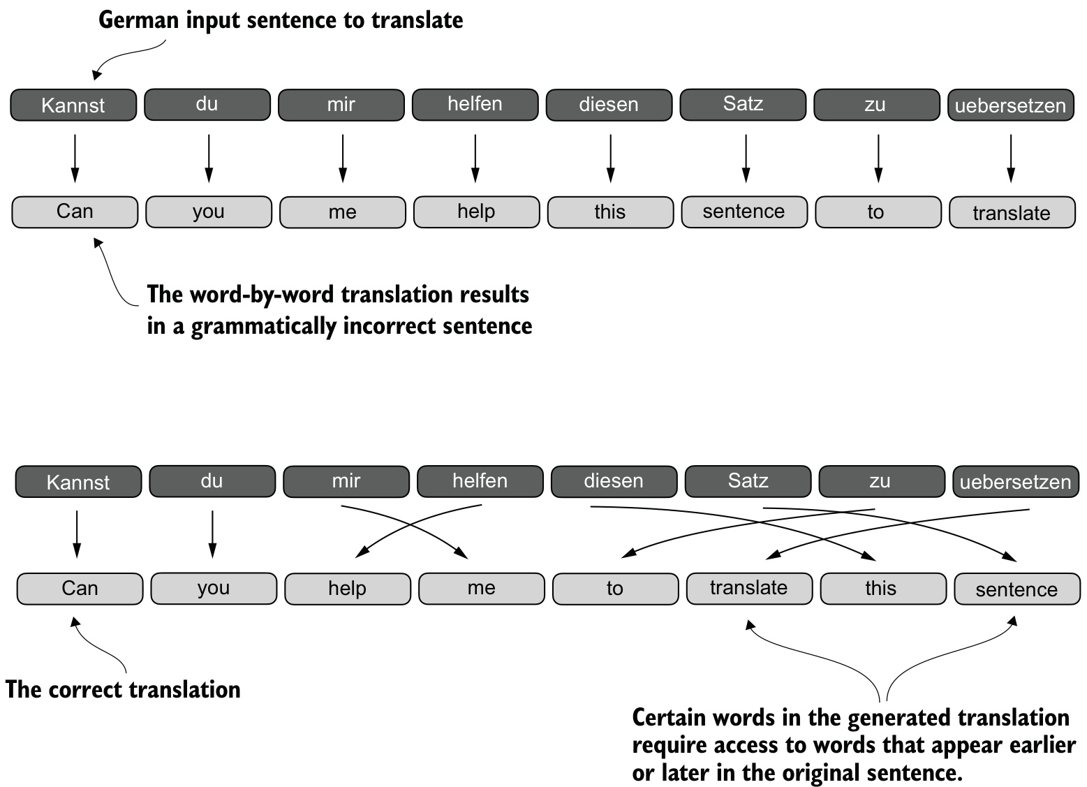
Machine translation is not word-by-word substitution. Translating the German sentence Kannst du mir helfen diesen Satz zu uebersetzen word by word yields Can you me help this sentence to translate, which is not English. The correct output, Can you help me translate this sentence, requires words that appear earlier or later in the source, so the generated sequence cannot be produced by a positional map from the input.
The standard pre-transformer answer was a deep network in two submodules, an encoder and a decoder. Before transformers, the most popular encoder-decoder architecture for translation used recurrent neural networks, in which outputs from previous steps are fed as inputs to the current step. The encoder reads the input text sequentially and updates its hidden state — the internal values at the hidden layers — at each step, attempting to capture the entire meaning of the input sentence in the final hidden state. The decoder takes that final hidden state and begins generating the translated sentence one word at a time, updating its own hidden state at each step.
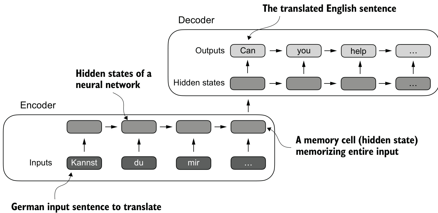
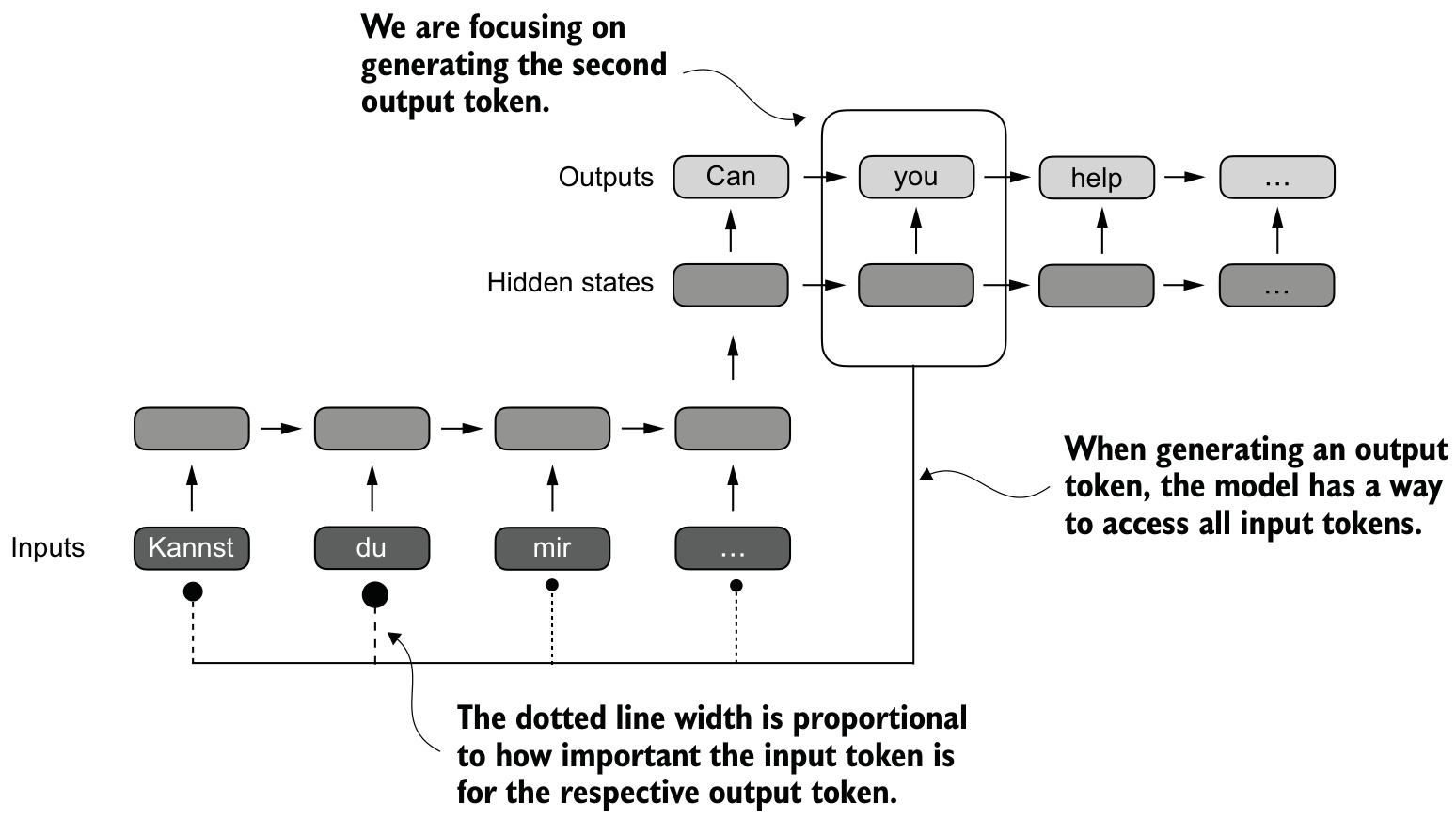
The limitation is a matter of access, not of capacity in principle. The RNN cannot directly access earlier hidden states from the encoder during the decoding phase; it relies solely on the current hidden state, which is required to encapsulate all relevant information. Context is lost in complex sentences where dependencies span long distances.
Bahdanau attention, developed for RNNs in 2014 and named after the first author of the paper, modifies the encoder-decoder RNN so that the decoder can selectively access different parts of the input sequence at each decoding step. The importance of each input token for a given output token is determined by attention weights. The single fixed-size hidden state is no longer the only channel between the two halves.
Three years later, researchers found that RNN architectures are not required for deep neural networks in natural language processing, and proposed the original transformer architecture with a self-attention mechanism inspired by Bahdanau attention. Self-attention allows each position in the input sequence to consider the relevancy of, or attend to, all other positions in the same sequence when computing the representation of that sequence.
The “self” refers to the mechanism’s ability to compute attention weights by relating different positions within a single input sequence. Traditional attention mechanisms focus on the relationships between elements of two different sequences, such as the input sequence and the output sequence in a sequence-to-sequence model.
Learning outcomes
- explain-rnn-bottleneck Explain the information bottleneck of RNN encoder-decoder models and how attention removes it.
Concepts
- self-attention succeeds the RNN and the Bahdanau mechanism by giving every position direct access to every other position in the same sequence
A simplified self-attention mechanism
Take an input sequence \(x\) of \(T\) elements, written \(x^{(1)}\) to \(x^{(T)}\), each a \(d\)-dimensional token embedding. The goal is a context vector \(z^{(i)}\) for every \(x^{(i)}\): an enriched embedding containing information about \(x^{(i)}\) and all the other input elements.
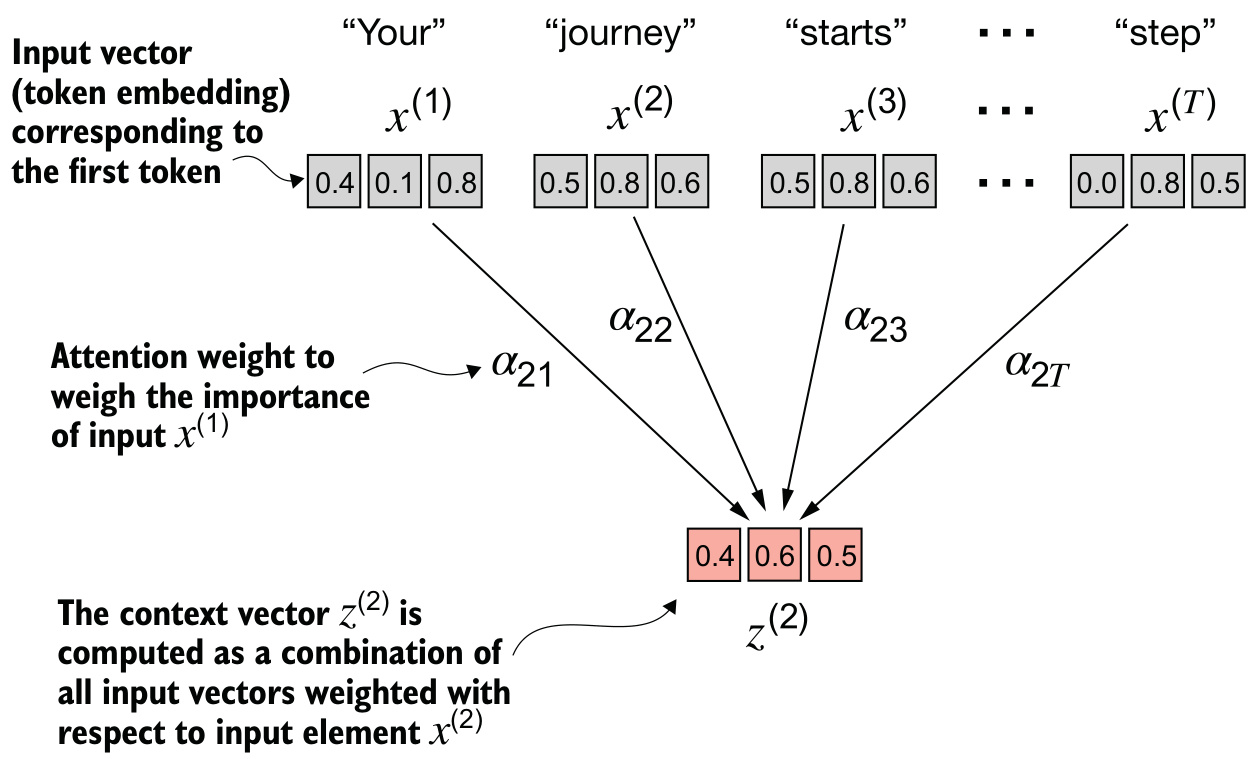
The worked sentence is “Your journey starts with one step.”, already embedded into three-dimensional vectors. The embedding dimension is small only so that the tensor fits on the page without line breaks.
import torch
inputs = torch.tensor(
  [[0.43, 0.15, 0.89], # Your     (x^1)
   [0.55, 0.87, 0.66], # journey  (x^2)
   [0.57, 0.85, 0.64], # starts   (x^3)
   [0.22, 0.58, 0.33], # with     (x^4)
   [0.77, 0.25, 0.10], # one      (x^5)
   [0.05, 0.80, 0.55]] # step     (x^6)
)
Step 1: attention scores
The second input element, \(x^{(2)}\) — the token “journey” — serves as the query. The intermediate values \(\omega\), the attention scores, are the dot products of the query with every input token.
query = inputs[1]
attn_scores_2 = torch.empty(inputs.shape[0])
for i, x_i in enumerate(inputs):
    attn_scores_2[i] = torch.dot(x_i, query)
print(attn_scores_2)
tensor([0.9544, 1.4950, 1.4754, 0.8434, 0.7070, 1.0865])A dot product multiplies two vectors element-wise and sums the products. Beyond that, it is a measure of similarity, because it quantifies how closely two vectors are aligned: the higher the dot product, the higher the similarity and attention score between two elements. The largest score, \(1.4950\), is the query with itself.
Step 2: attention weights
The scores are normalized so that they sum to \(1\), a convention useful for interpretation and for maintaining training stability. Dividing by the sum achieves it, but the softmax function is more common and advisable, being better at managing extreme values and offering more favourable gradient properties during training.
def softmax_naive(x):
    return torch.exp(x) / torch.exp(x).sum(dim=0)

attn_weights_2_naive = softmax_naive(attn_scores_2)
Attention weights: tensor([0.1385, 0.2379, 0.2333, 0.1240, 0.1082, 0.1581])
Sum: tensor(1.)Softmax also guarantees positive weights, which makes the output interpretable as probabilities or relative importance.
softmax_naive may encounter numerical instability problems, such as overflow and underflow, when dealing with large or small input values. The PyTorch implementation, torch.softmax(attn_scores_2, dim=0), has been extensively optimized for performance and yields the same result here.
Step 3: the context vector
The context vector \(z^{(2)}\) is the weighted sum of all input vectors, each multiplied by its corresponding attention weight.
query = inputs[1]
context_vec_2 = torch.zeros(query.shape)
for i,x_i in enumerate(inputs):
    context_vec_2 += attn_weights_2[i]*x_i
print(context_vec_2)
tensor([0.4419, 0.6515, 0.5683])Nothing in these three steps is learned. The weights follow entirely from the input embeddings.
Learning outcomes
- compute-context-vector Compute a context vector for one query token with the three-step attention pipeline and no trainable weights.
Concepts
- self-attention produces one enriched context vector per token by dot products and softmax alone, with no trainable parameters
- dot-product-similarity the dot product of a query with an input measures their alignment, and serves directly as the unnormalized attention score
Computing attention weights for all input tokens
The single query of the previous section is one row of a square matrix. Every other row is another token used as the query.
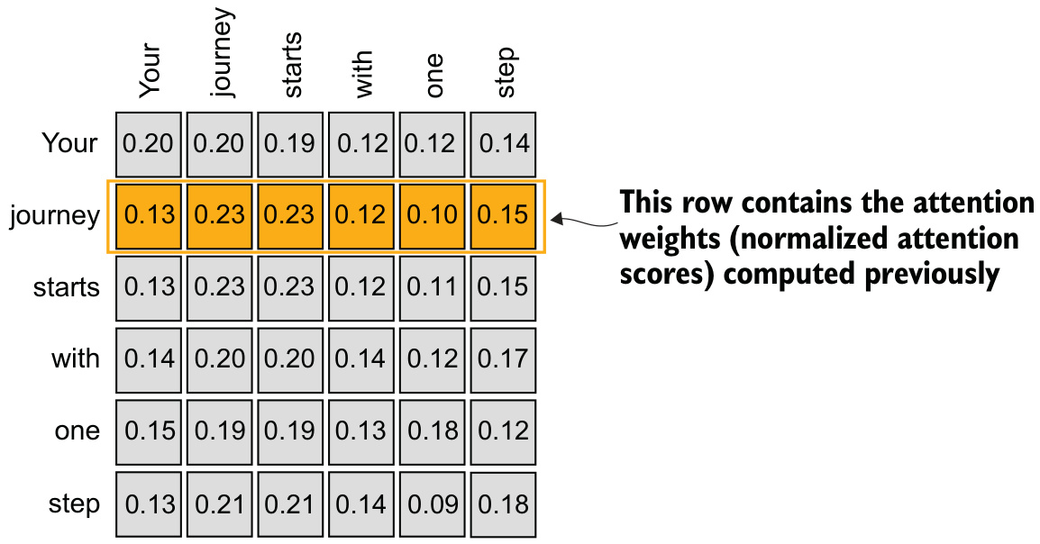
The same three steps, with an added for loop over query positions, produce the full score matrix.
attn_scores = torch.empty(6, 6)
for i, x_i in enumerate(inputs):
    for j, x_j in enumerate(inputs):
        attn_scores[i, j] = torch.dot(x_i, x_j)
print(attn_scores)
tensor([[0.9995, 0.9544, 0.9422, 0.4753, 0.4576, 0.6310],
[0.9544, 1.4950, 1.4754, 0.8434, 0.7070, 1.0865],
[0.9422, 1.4754, 1.4570, 0.8296, 0.7154, 1.0605],
[0.4753, 0.8434, 0.8296, 0.4937, 0.3474, 0.6565],
[0.4576, 0.7070, 0.7154, 0.3474, 0.6654, 0.2935],
[0.6310, 1.0865, 1.0605, 0.6565, 0.2935, 0.9450]])for loops are generally slow, and the same result is achieved with one matrix multiplication.
attn_scores = inputs @ inputs.TEntry \((i, j)\) of attn_scores is the dot product of token \(i\) with token \(j\). The second row is exactly the attn_scores_2 computed before.
Normalization is applied row-wise.
attn_weights = torch.softmax(attn_scores, dim=-1)tensor([[0.2098, 0.2006, 0.1981, 0.1242, 0.1220, 0.1452],
[0.1385, 0.2379, 0.2333, 0.1240, 0.1082, 0.1581],
[0.1390, 0.2369, 0.2326, 0.1242, 0.1108, 0.1565],
[0.1435, 0.2074, 0.2046, 0.1462, 0.1263, 0.1720],
[0.1526, 0.1958, 0.1975, 0.1367, 0.1879, 0.1295],
[0.1385, 0.2184, 0.2128, 0.1420, 0.0988, 0.1896]])The dim parameter in torch.softmax specifies the dimension of the input tensor along which the function is computed. Setting dim=-1 applies the normalization along the last dimension of attn_scores. For a two-dimensional tensor of shape [rows, columns], it normalizes across the columns, so the values in each row sum to \(1\). The check is one line:
print("All row sums:", attn_weights.sum(dim=-1))All row sums: tensor([1.0000, 1.0000, 1.0000, 1.0000, 1.0000, 1.0000])The third step is another matrix multiplication.
all_context_vecs = attn_weights @ inputstensor([[0.4421, 0.5931, 0.5790],
[0.4419, 0.6515, 0.5683],
[0.4431, 0.6496, 0.5671],
[0.4304, 0.6298, 0.5510],
[0.4671, 0.5910, 0.5266],
[0.4177, 0.6503, 0.5645]])Each row is a three-dimensional context vector. The second row, [0.4419, 0.6515, 0.5683], matches context_vec_2 from the loop exactly, which is the correctness check on the vectorized form.
Learning outcomes
- vectorize-over-all-tokens Vectorize the attention computation so every token gets its context vector in one matrix operation.
Concepts
- self-attention all context vectors are obtained concurrently as
attn_weights @ inputs, one row per token - dot-product-similarity the full matrix of pairwise dot products is
inputs @ inputs.T, replacing the nested loops
Self-attention with trainable weights
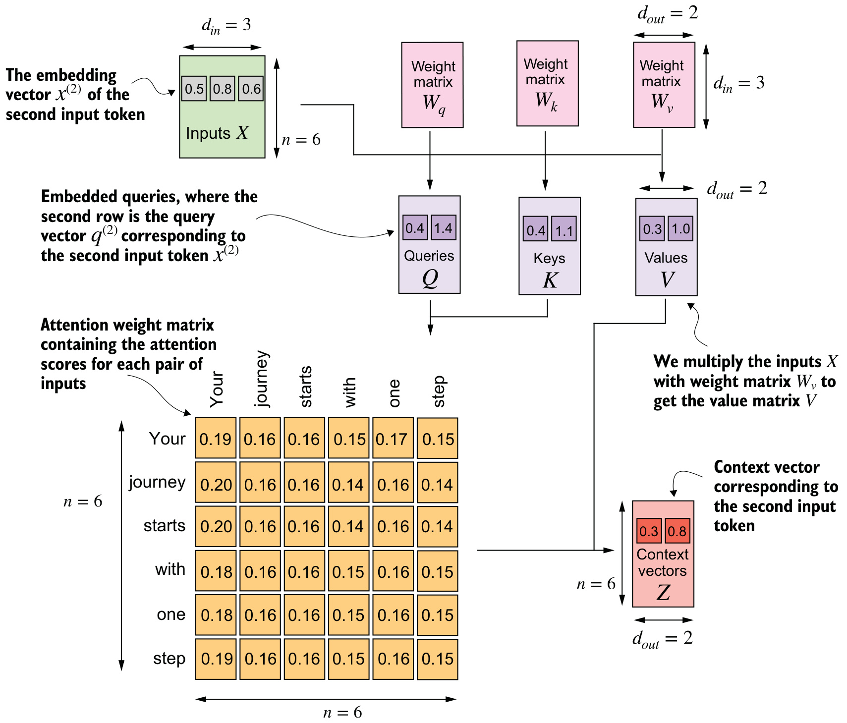
The mechanism used in the original transformer architecture, the GPT models and most other popular LLMs is called scaled dot-product attention. It differs from the simplified version by the introduction of weight matrices that are updated during model training, so that the model can learn to produce good context vectors.
Three trainable weight matrices \(W_q\), \(W_k\) and \(W_v\) project each embedded input token \(x^{(i)}\) into a query, a key and a value vector.
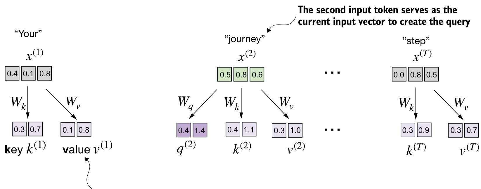
x_2 = inputs[1]
d_in = inputs.shape[1]
d_out = 2
In GPT-like models the input and output dimensions are usually the same; here d_in=3 and d_out=2 differ so that the shapes in the computation can be told apart.
torch.manual_seed(123)
W_query = torch.nn.Parameter(torch.rand(d_in, d_out), requires_grad=False)
W_key   = torch.nn.Parameter(torch.rand(d_in, d_out), requires_grad=False)
W_value = torch.nn.Parameter(torch.rand(d_in, d_out), requires_grad=False)
requires_grad=False reduces clutter in the outputs; training the matrices requires requires_grad=True.
query_2 = x_2 @ W_query
key_2 = x_2 @ W_key
value_2 = x_2 @ W_value
tensor([0.4306, 1.4551])Computing \(z^{(2)}\) alone still requires the key and value vectors for all input elements, since they take part in the attention weights with respect to \(q^{(2)}\).
keys = inputs @ W_key
values = inputs @ W_value
keys.shape: torch.Size([6, 2])
values.shape: torch.Size([6, 2])In \(W_q\), \(W_k\) and \(W_v\), “weight” is short for “weight parameters”: the values of a neural network that are optimized during training. They are the fundamental, learned coefficients that define the network’s connections. Attention weights determine the extent to which a context vector depends on the different parts of the input, and are dynamic, context-specific values recomputed for every input sequence.
The score is now a dot product of query and key
keys_2 = keys[1]
attn_score_22 = query_2.dot(keys_2)tensor(1.8524)Generalized to all keys for that one query:
attn_scores_2 = query_2 @ keys.Ttensor([1.2705, 1.8524, 1.8111, 1.0795, 0.5577, 1.5440])The scaling by \(\sqrt{d_k}\)
The scores are divided by the square root of the embedding dimension of the keys before the softmax. Taking the square root is mathematically the same as exponentiating by \(0.5\).
d_k = keys.shape[-1]
attn_weights_2 = torch.softmax(attn_scores_2 / d_k**0.5, dim=-1)
tensor([0.1500, 0.2264, 0.2199, 0.1311, 0.0906, 0.1820])The reason for normalizing by the embedding dimension size is to improve training performance by avoiding small gradients. When scaling up the embedding dimension — typically greater than \(1{,}000\) for GPT-like LLMs — large dot products can result in very small gradients during backpropagation, because of the softmax applied to them. As dot products increase, the softmax function behaves more like a step function, resulting in gradients nearing zero. These small gradients can drastically slow down learning or cause training to stagnate. The scaling by the square root of the embedding dimension is the reason this mechanism is called scaled dot-product attention.
The context vector is a weighted sum of values
context_vec_2 = attn_weights_2 @ valuestensor([0.3061, 0.8210])The sum runs over the value vectors, not over the raw inputs. The attention weights serve as a weighting factor that weighs the respective importance of each value vector.
The terms come from information retrieval. A query is analogous to a search query: the item the model currently focuses on. A key is like a database key used for indexing and searching, matched against the query. A value is like the value in a key-value pair: the actual content retrieved once the model has determined which keys are most relevant to the query.
Learning outcomes
- implement-trainable-attention Implement self-attention with trainable query, key and value projection matrices and scaled dot products.
Concepts
- self-attention becomes learnable once the fixed embeddings are replaced by three projections that gradient descent updates
- qkv-projections \(W_q\), \(W_k\) and \(W_v\) map each input into the item being looked up, the index it is matched against, and the content aggregated into the context vector
- dot-product-similarity the score \(\omega\) is now \(q \cdot k\), a dot product between two projected vectors rather than between two raw embeddings
- scaled-dot-product-attention dividing the scores by \(\sqrt{d_k}\) before the softmax keeps the distribution away from the saturated region where gradients vanish
A compact self-attention class
The loose tensor code becomes a subclass of nn.Module, the fundamental building block of PyTorch models, which provides the functionality for model layer creation and management. __init__ holds the three weight matrices; forward holds the computation.
import torch.nn as nn
class SelfAttention_v1(nn.Module):
    def __init__(self, d_in, d_out):
        super().__init__()
        self.W_query = nn.Parameter(torch.rand(d_in, d_out))
        self.W_key   = nn.Parameter(torch.rand(d_in, d_out))
        self.W_value = nn.Parameter(torch.rand(d_in, d_out))

    def forward(self, x):
        keys = x @ self.W_key
        queries = x @ self.W_query
        values = x @ self.W_value
        attn_scores = queries @ keys.T # omega
        attn_weights = torch.softmax(
            attn_scores / keys.shape[-1]**0.5, dim=-1
        )
        context_vec = attn_weights @ values
        return context_vec
Applied to the six input embeddings, the module returns six context vectors, and the second row [0.3061, 0.8210] matches the context_vec_2 computed by hand.
nn.Linear layers effectively perform matrix multiplication when the bias units are disabled, and a significant advantage of using nn.Linear instead of manually implementing nn.Parameter(torch.rand(...)) is that nn.Linear has an optimized weight initialization scheme, contributing to more stable and effective model training.
class SelfAttention_v2(nn.Module):
    def __init__(self, d_in, d_out, qkv_bias=False):
        super().__init__()
        self.W_query = nn.Linear(d_in, d_out, bias=qkv_bias)
        self.W_key   = nn.Linear(d_in, d_out, bias=qkv_bias)
        self.W_value = nn.Linear(d_in, d_out, bias=qkv_bias)

    def forward(self, x):
        keys = self.W_key(x)
        queries = self.W_query(x)
        values = self.W_value(x)
        attn_scores = queries @ keys.T
        attn_weights = torch.softmax(
            attn_scores / keys.shape[-1]**0.5, dim=-1
        )
        context_vec = attn_weights @ values
        return context_vec
tensor([[-0.0739, 0.0713],
[-0.0748, 0.0703],
[-0.0749, 0.0702],
[-0.0760, 0.0685],
[-0.0763, 0.0679],
[-0.0754, 0.0693]], grad_fn=<MmBackward0>)SelfAttention_v1 and SelfAttention_v2 give different outputs because they use different initial weights for the weight matrices, nn.Linear using a more sophisticated weight initialization scheme. The two compute the same function of their parameters; they do not start from the same parameters.
The two implementations are otherwise similar, so the weight matrices from a SelfAttention_v2 object can be transferred to a SelfAttention_v1 such that both objects then produce the same results. The task is to assign the weights correctly. Hint from the source: nn.Linear stores the weight matrix in a transposed form.
Learning outcomes
- package-attention-module Package self-attention as a compact
nn.Module, usingnn.Linearrather than rawnn.Parameter. - implement-trainable-attention Implement self-attention with trainable query, key and value projection matrices and scaled dot products.
Concepts
- self-attention packaged as an
nn.Module, it becomes a reusable layer that later refinements edit rather than rewrite - qkv-projections the three projections live in
__init__, either asnn.Parametertensors or as bias-freenn.Linearlayers - scaled-dot-product-attention the whole scaled formula sits inside
forward, dividing bykeys.shape[-1]**0.5before the softmax
Hiding future words with causal attention
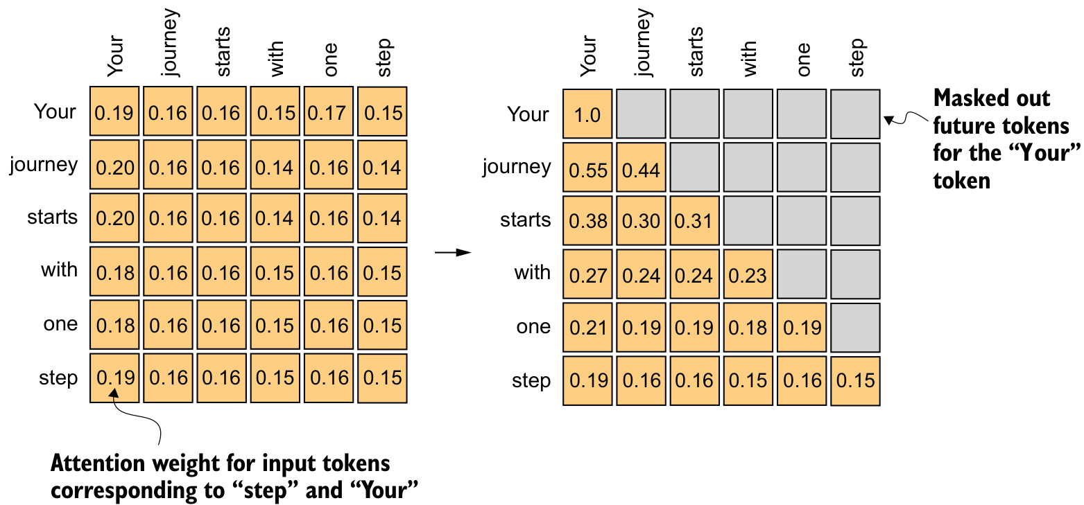
For many LLM tasks the self-attention mechanism must consider only the tokens that appear prior to the current position when predicting the next token in a sequence. Causal attention, also known as masked attention, is a specialized form of self-attention that restricts a model to only consider previous and current inputs in a sequence when computing attention scores. This is in contrast to the standard self-attention mechanism, which allows access to the entire input sequence at once.
Masking after the softmax
Starting from the attention weights of the previous section, torch.tril builds a mask whose values above the diagonal are zero.
context_length = attn_scores.shape[0]
mask_simple = torch.tril(torch.ones(context_length, context_length))
masked_simple = attn_weights*mask_simple
The rows of masked_simple no longer sum to \(1\), so a third step divides each element in a row by the sum in that row.
row_sums = masked_simple.sum(dim=-1, keepdim=True)
masked_simple_norm = masked_simple / row_sums
tensor([[1.0000, 0.0000, 0.0000, 0.0000, 0.0000, 0.0000],
[0.5517, 0.4483, 0.0000, 0.0000, 0.0000, 0.0000],
[0.3800, 0.3097, 0.3103, 0.0000, 0.0000, 0.0000],
[0.2758, 0.2460, 0.2462, 0.2319, 0.0000, 0.0000],
[0.2175, 0.1983, 0.1984, 0.1888, 0.1971, 0.0000],
[0.1935, 0.1663, 0.1666, 0.1542, 0.1666, 0.1529]],
grad_fn=<DivBackward0>)It might appear that information from the masked future tokens still influences the current token, because their values were part of the softmax calculation. Renormalizing the attention weights after masking is recalculating the softmax over a smaller subset, since masked positions do not contribute to the softmax value. Despite initially including all positions in the denominator, after masking and renormalizing the effect of the masked positions is nullified. The resulting distribution is as if it had been calculated only among the unmasked positions to begin with.
Masking before the softmax
The softmax function converts its inputs into a probability distribution. When negative infinity values are present in a row, the softmax function treats them as zero probability, because \(e^{-\infty}\) approaches \(0\). That makes the mask applicable to the scores, in fewer steps.
mask = torch.triu(torch.ones(context_length, context_length), diagonal=1)
masked = attn_scores.masked_fill(mask.bool(), -torch.inf)
tensor([[0.2899, -inf, -inf, -inf, -inf, -inf],
[0.4656, 0.1723, -inf, -inf, -inf, -inf],
[0.4594, 0.1703, 0.1731, -inf, -inf, -inf],
[0.2642, 0.1024, 0.1036, 0.0186, -inf, -inf],
[0.2183, 0.0874, 0.0882, 0.0177, 0.0786, -inf],
[0.3408, 0.1270, 0.1290, 0.0198, 0.1290, 0.0078]],
grad_fn=<MaskedFillBackward0>)attn_weights = torch.softmax(masked / keys.shape[-1]**0.5, dim=1)The values in each row sum to \(1\), and no further normalization is necessary. The result is identical to masked_simple_norm. Note that diagonal=1 in torch.triu is what excludes the main diagonal from the mask: a token must still attend to itself.
Learning outcomes
- apply-causal-mask Apply a causal mask so that no token can attend to a token that follows it.
Concepts
- causal-attention
torch.triu(..., diagonal=1)marks the strictly future positions, andmasked_fillsets those scores to-torch.infbefore the softmax, which sends their weights to zero without a second normalization pass
Masking additional attention weights with dropout
Dropout in deep learning is a technique where randomly selected hidden layer units are ignored during training, effectively dropping them out. It helps prevent overfitting by ensuring that a model does not become overly reliant on any specific set of hidden layer units. Dropout is only used during training and is disabled afterward.
In the transformer architecture, including models like GPT, dropout in the attention mechanism is typically applied at two specific times: after calculating the attention weights, or after applying the attention weights to the value vectors. Applying it after computing the attention weights is the more common variant in practice.
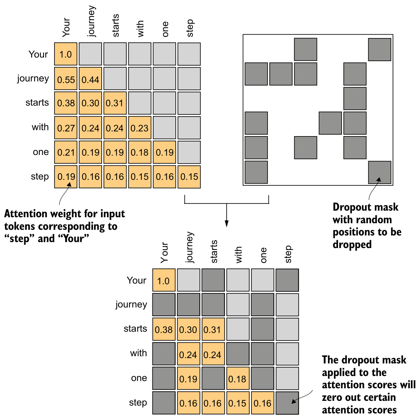
The illustration uses a dropout rate of 50%, which means masking out half of the attention weights. Training the GPT model in later chapters uses a lower rate, such as \(0.1\) or \(0.2\). Applied first to a \(6 \times 6\) tensor of ones:
torch.manual_seed(123)
dropout = torch.nn.Dropout(0.5)
example = torch.ones(6, 6)
print(dropout(example))
tensor([[2., 2., 0., 2., 2., 0.],
[0., 0., 0., 2., 0., 2.],
[2., 2., 2., 2., 0., 2.],
[0., 2., 2., 0., 0., 2.],
[0., 2., 0., 2., 0., 2.],
[0., 2., 2., 2., 2., 0.]])Approximately half the values are zeroed out. To compensate for the reduction in active elements, the values of the remaining elements in the matrix are scaled up by a factor of \(1/0.5 = 2\). This scaling is crucial to maintain the overall balance of the attention weights, ensuring that the average influence of the attention mechanism remains consistent during both the training and inference phases. That factor is why the surviving entries read \(2\) rather than \(1\).
Applied to the causally masked attention weight matrix:
torch.manual_seed(123)
print(dropout(attn_weights))
tensor([[2.0000, 0.0000, 0.0000, 0.0000, 0.0000, 0.0000],
[0.0000, 0.0000, 0.0000, 0.0000, 0.0000, 0.0000],
[0.7599, 0.6194, 0.6206, 0.0000, 0.0000, 0.0000],
[0.0000, 0.4921, 0.4925, 0.0000, 0.0000, 0.0000],
[0.0000, 0.3966, 0.0000, 0.3775, 0.0000, 0.0000],
[0.0000, 0.3327, 0.3331, 0.3084, 0.3331, 0.0000]],
grad_fn=<MulBackward0>)The resulting dropout outputs may look different depending on the operating system. The source records the inconsistency at the PyTorch issue tracker, https://github.com/pytorch/pytorch/issues/121595. Reproducing the printed tensor exactly is not the point of the exercise; the pattern of zeros and the factor of \(2\) are.
Learning outcomes
- apply-attention-dropout Regularize attention with dropout, and account for the rescaling it applies.
Concepts
- attention-dropout dropout on the normalized attention weight matrix zeroes a random fraction \(p\) of the connections during training and scales the survivors by \(1/(1-p)\)
A compact causal attention class
Real training data arrives from the data loader in batches, so the class must accept a three-dimensional tensor. Duplicating the input simulates one:
batch = torch.stack((inputs, inputs), dim=0)
print(batch.shape)
torch.Size([2, 6, 3])Two input texts with six tokens each, each token a three-dimensional embedding.
class CausalAttention(nn.Module):
    def __init__(self, d_in, d_out, context_length,
                 dropout, qkv_bias=False):
        super().__init__()
        self.d_out = d_out
        self.W_query = nn.Linear(d_in, d_out, bias=qkv_bias)
        self.W_key   = nn.Linear(d_in, d_out, bias=qkv_bias)
        self.W_value = nn.Linear(d_in, d_out, bias=qkv_bias)
        self.dropout = nn.Dropout(dropout)
        self.register_buffer(
           'mask',
           torch.triu(torch.ones(context_length, context_length),
           diagonal=1)
        )

    def forward(self, x):
        b, num_tokens, d_in = x.shape
        keys = self.W_key(x)
        queries = self.W_query(x)
        values = self.W_value(x)

        attn_scores = queries @ keys.transpose(1, 2)
        attn_scores.masked_fill_(
            self.mask.bool()[:num_tokens, :num_tokens], -torch.inf)
        attn_weights = torch.softmax(
            attn_scores / keys.shape[-1]**0.5, dim=-1
        )
        attn_weights = self.dropout(attn_weights)

        context_vec = attn_weights @ values
        return context_vec
Three details separate this from SelfAttention_v2.
The score computation is
queries @ keys.transpose(1, 2), notqueries @ keys.T.transpose(1, 2)exchanges dimensions 1 and 2, keeping the batch dimension at the first position, position 0..Twould transpose all axes and break the batch.The mask is held by
register_buffer.Using
register_bufferis not strictly necessary for all use cases, but buffers are automatically moved to the appropriate device, CPU or GPU, along with the model. There is then no need to manually ensure these tensors are on the same device as the model parameters, which avoids device mismatch errors.The mask is sliced to
[:num_tokens, :num_tokens]insideforward.The buffer is built once at
context_length. A batch may carry fewer tokens than that, and the slice is what lets the same module serve a shorter sequence.
masked_fill_ carries a trailing underscore: in PyTorch, operations with a trailing underscore are performed in place, avoiding unnecessary memory copies.
torch.manual_seed(123)
context_length = batch.shape[1]
ca = CausalAttention(d_in, d_out, context_length, 0.0)
context_vecs = ca(batch)
print("context_vecs.shape:", context_vecs.shape)
context_vecs.shape: torch.Size([2, 6, 2])Each of the six tokens in each of the two sequences is now represented by a two-dimensional embedding.
Learning outcomes
- handle-batched-inputs Write an attention module that handles batched inputs of shape (batch, tokens, dimension).
- apply-causal-mask Apply a causal mask so that no token can attend to a token that follows it.
- apply-attention-dropout Regularize attention with dropout, and account for the rescaling it applies.
- package-attention-module Package self-attention as a compact
nn.Module, usingnn.Linearrather than rawnn.Parameter.
Concepts
- causal-attention the triangular mask becomes registered module state, sliced to the batch’s token count on every forward pass
- attention-dropout an
nn.Dropoutlayer sits between the softmax and the multiplication by the values - qkv-projections the three
nn.Linearlayers project a batched tensor of shape (batch, tokens,d_in) into queries, keys and values
Stacking multiple single-head attention layers
The term multi-head attention refers to dividing the attention mechanism into multiple heads, each operating independently. A single causal attention module is single-head attention: one set of attention weights processing the input sequentially.
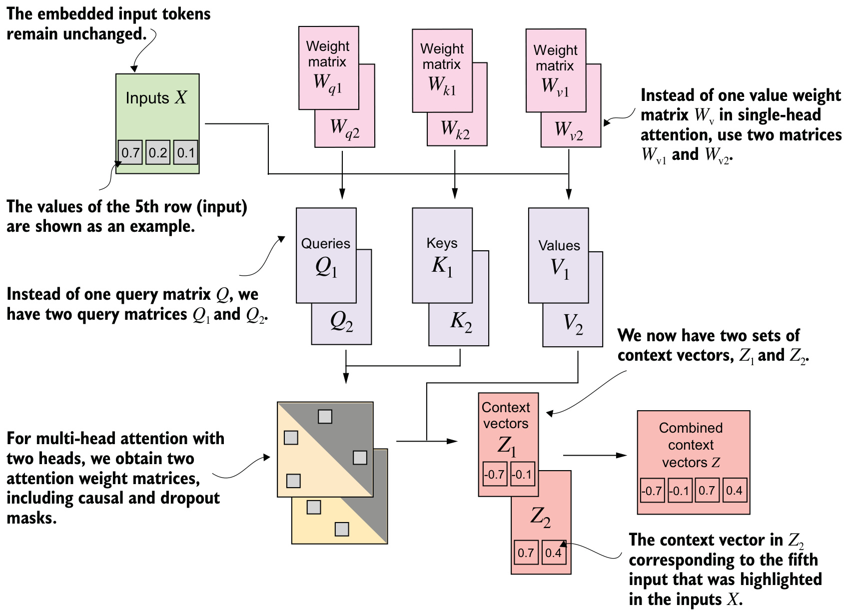
The main idea is to run the attention mechanism multiple times, in parallel, with different learned linear projections. In code, that is a wrapper holding multiple instances of CausalAttention.
class MultiHeadAttentionWrapper(nn.Module):
    def __init__(self, d_in, d_out, context_length,
                 dropout, num_heads, qkv_bias=False):
        super().__init__()
        self.heads = nn.ModuleList(
            [CausalAttention(
                 d_in, d_out, context_length, dropout, qkv_bias
             )
             for _ in range(num_heads)]
        )

    def forward(self, x):
        return torch.cat([head(x) for head in self.heads], dim=-1)
With num_heads=2 and CausalAttention output dimension d_out=2, the result is a four-dimensional context vector, d_out*num_heads=4.
torch.manual_seed(123)
context_length = batch.shape[1] # This is the number of tokens
d_in, d_out = 3, 2
mha = MultiHeadAttentionWrapper(
    d_in, d_out, context_length, 0.0, num_heads=2
)
context_vecs = mha(batch)
context_vecs.shape: torch.Size([2, 6, 4])The first dimension is \(2\) because there are two input texts, which were duplicated, which is why the context vectors are exactly the same for those. The second refers to the six tokens in each input. The third is the four-dimensional embedding of each token.
The cost is in the forward method: the heads are processed sequentially via [head(x) for head in self.heads], and each head repeats the matrix multiplication that computes its keys, queries and values.
Change the input arguments to the MultiHeadAttentionWrapper(..., num_heads=2) call so that the output context vectors are two-dimensional instead of four-dimensional, while keeping the setting num_heads=2. The class implementation does not need to change; only one of the other input arguments does.
Learning outcomes
- implement-multi-head-attention Implement multi-head causal attention, first by stacking heads and then by splitting one large projection.
Concepts
- multi-head-attention an
nn.ModuleListof independent heads whose context vectors are concatenated along the last dimension, giving an output width ofd_outtimesnum_heads - causal-attention each head is a complete
CausalAttentioninstance with its own mask, dropout and projections
Multi-head attention with weight splits
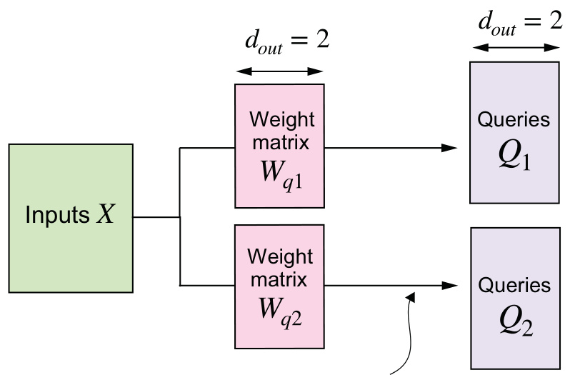
The MultiHeadAttention class integrates the multi-head functionality within a single class. It splits the input into multiple heads by reshaping the projected query, key and value tensors, then combines the results from these heads after computing attention.
class MultiHeadAttention(nn.Module):
    def __init__(self, d_in, d_out,
                 context_length, dropout, num_heads, qkv_bias=False):
        super().__init__()
        assert (d_out % num_heads == 0), \
            "d_out must be divisible by num_heads"

        self.d_out = d_out
        self.num_heads = num_heads
        self.head_dim = d_out // num_heads
        self.W_query = nn.Linear(d_in, d_out, bias=qkv_bias)
        self.W_key = nn.Linear(d_in, d_out, bias=qkv_bias)
        self.W_value = nn.Linear(d_in, d_out, bias=qkv_bias)
        self.out_proj = nn.Linear(d_out, d_out)
        self.dropout = nn.Dropout(dropout)
        self.register_buffer(
            "mask",
            torch.triu(torch.ones(context_length, context_length),
                       diagonal=1)
        )

    def forward(self, x):
        b, num_tokens, d_in = x.shape
        keys = self.W_key(x)
        queries = self.W_query(x)
        values = self.W_value(x)

        keys = keys.view(b, num_tokens, self.num_heads, self.head_dim)
        values = values.view(b, num_tokens, self.num_heads, self.head_dim)
        queries = queries.view(
            b, num_tokens, self.num_heads, self.head_dim
        )

        keys = keys.transpose(1, 2)
        queries = queries.transpose(1, 2)
        values = values.transpose(1, 2)

        attn_scores = queries @ keys.transpose(2, 3)
        mask_bool = self.mask.bool()[:num_tokens, :num_tokens]

        attn_scores.masked_fill_(mask_bool, -torch.inf)

        attn_weights = torch.softmax(
            attn_scores / keys.shape[-1]**0.5, dim=-1)
        attn_weights = self.dropout(attn_weights)

        context_vec = (attn_weights @ values).transpose(1, 2)

        context_vec = context_vec.contiguous().view(
            b, num_tokens, self.d_out
        )
        context_vec = self.out_proj(context_vec)
        return context_vec
The key operation is to split the d_out dimension into num_heads and head_dim, where head_dim = d_out / num_heads. The .view method reshapes a tensor of dimensions (b, num_tokens, d_out) to (b, num_tokens, num_heads, head_dim). The assert at the top of __init__ is what enforces divisibility.
The tensors are then transposed to bring the num_heads dimension before the num_tokens dimension, giving shape (b, num_heads, num_tokens, head_dim). This transposition is crucial for correctly aligning the queries, keys and values across the different heads and performing batched matrix multiplications efficiently. PyTorch carries out the matrix multiplication between the two last dimensions, num_tokens and head_dim, and repeats it for the individual heads. Slicing out a[0, 0, :, :] and computing first_head @ first_head.T gives exactly what a @ a.transpose(2, 3) produces for that head.
After computing the attention weights and context vectors, the context vectors from all heads are transposed back to the shape (b, num_tokens, num_heads, head_dim) and reshaped, flattened, into the shape (b, num_tokens, d_out), effectively combining the outputs from all heads. The output projection layer self.out_proj is added after combining the heads, and is not present in the CausalAttention class. It is not strictly necessary but is commonly used in many LLM architectures.
The reason this is more efficient than the wrapper is that only one matrix multiplication is needed to compute the keys, keys = self.W_key(x), and the same holds for the queries and values. In the MultiHeadAttentionWrapper that matrix multiplication — computationally one of the most expensive steps — is repeated for each attention head.
torch.manual_seed(123)
batch_size, context_length, d_in = batch.shape
d_out = 2
mha = MultiHeadAttention(d_in, d_out, context_length, 0.0, num_heads=2)
context_vecs = mha(batch)
context_vecs.shape: torch.Size([2, 6, 2])The output dimension is directly controlled by the d_out argument, so unlike the wrapper the width does not grow with the number of heads.
The embedding sizes and head counts used above are small to keep the printed tensors readable. The smallest GPT-2 model, 117 million parameters, has 12 attention heads and a context vector embedding size of 768. The largest GPT-2 model, 1.5 billion parameters, has 25 attention heads and a context vector embedding size of 1,600. The embedding sizes of the token inputs and context embeddings are the same in GPT models, d_in = d_out.
Using the MultiHeadAttention class, initialize a multi-head attention module with the same number of attention heads as the smallest GPT-2 model, 12 attention heads, and input and output embedding sizes similar to GPT-2, 768 dimensions. The smallest GPT-2 model supports a context length of 1,024 tokens.
Learning outcomes
- implement-multi-head-attention Implement multi-head causal attention, first by stacking heads and then by splitting one large projection.
- handle-batched-inputs Write an attention module that handles batched inputs of shape (batch, tokens, dimension).
Concepts
- multi-head-attention one projection of width
d_outis reshaped with.viewand.transposeintonum_headsslices of widthhead_dim, and every head’s scores are computed by a single batched matrix multiplication - qkv-projections
W_query,W_keyandW_valueeach serve all heads at once, andout_projrecombines their concatenated outputs - causal-attention the registered mask, sliced to
num_tokens, applies across the four-dimensional score tensor for all heads simultaneously - attention-dropout the same dropout layer regularizes the four-dimensional attention weight tensor across every head
Key ideas
Attention mechanisms overcome the information bottleneck of the RNN encoder-decoder model.
The decoder of an encoder-decoder RNN cannot directly access the encoder’s earlier hidden states, so everything the source contributes must fit in one final hidden state. Attention gives the decoder weighted access to every input position instead.
Self-attention computes the context vector representation as a weighted sum over the inputs, in three steps.
Scores are dot products, weights are the softmax of those scores along the sequence dimension, and the context vector is the weighted sum. Trainable attention replaces the raw inputs by projected values and divides the scores by \(\sqrt{d_k}\) first.
Matrix multiplication replaces the nested
forloops without changing the result.inputs @ inputs.T, a row-wisesoftmax(dim=-1), andattn_weights @ inputsreproduce the looped context vectors exactly, andqueries @ keys.transpose(1, 2)extends that to a batch.Causal masking and dropout are the two masks a GPT-style attention layer applies.
Filling the strictly upper-triangular scores with
-torch.infbefore the softmax gives future positions exactly zero weight while the rows still sum to \(1\). Dropout then zeroes a random fraction of the surviving weights during training and scales the rest by \(1/(1-p)\).Multi-head attention is more efficient as one class than as a list of heads.
Both forms compute the same function. Projecting once at width
d_outand splitting with.viewand.transposeperforms one matrix multiplication per projection rather than one per head, and the head axis then rides along as a batch dimension.
The next unit, 4 Implementing a GPT model from scratch to generate text, treats the MultiHeadAttention class as one sub-layer of a transformer block. The rest of that block — a LayerNorm with learnable scale and shift, a GELU feed-forward network that expands 768 to 3072 and contracts back, pre-normalization, dropout and residual shortcut connections — is added around it, the block is repeated twelve times, and the resulting GPT-2 124M architecture is run through a greedy autoregressive loop that turns logits into text.
References
- Building a Large Language Model (from scratch), Sebastian Raschka, 2024, Manning Books — Link — Page 72-113