3 Coding attention mechanisms

Language Models · v1.0.0

2026-08-25 14:45:14

Where we are

From tokens to context

• The previous unit built the input pipeline: tokens, byte pair encoding, sliding-window batches, token + positional embeddings.
• That pipeline hands us a tensor of shape (batch, tokens, embedding dimension).
• This unit builds the layer that consumes it: attention.

Frame this as a direct continuation. We are not starting a new topic, we are building the next stage of the same pipeline.

Four passes over the same idea

We build attention in four passes, each keeping everything from the pass before.

1. Simplified self-attention — no trainable weights.
2. Trainable self-attention — query, key, value projections.
3. Causal self-attention — a mask over future tokens.
4. Multi-head attention — several attention operations in parallel.

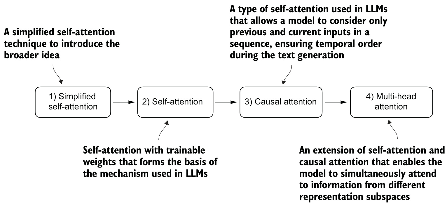
The attention variants we will code.

By the end of the unit these four passes combine into the MultiHeadAttention module the GPT model in the next unit drops into place.

What we will cover

• Self-attention — relates all positions within one sequence.
• Dot-product attention score — measures alignment between two vectors.
• Query, key, value projections — trainable maps into three roles.
• Scaled dot-product attention — scores divided by \(\sqrt{d_k}\).
• Causal attention — forbids attending to future tokens.
• Attention weight dropout — regularizes the normalized weights.
• Multi-head attention — several attention operations in parallel.

This unit is about the mechanism and its design rationale, not the full transformer block — that is Chapter 12: Transformers. For full working code and tensor-by-tensor detail, point students to Raschka chapter 3.

The long-sequence problem

Translation is not word-by-word

• Source and target languages do not put their words in the same order.
• Word-by-word translation cannot capture that.

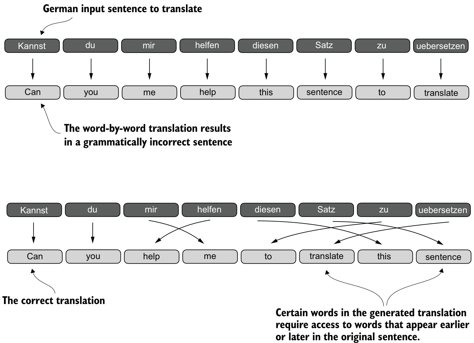
Translating German to English requires contextual and grammatical alignment.

The encoder-decoder bottleneck

• Before transformers: an encoder and a decoder, often built from RNNs.
• The encoder compresses the entire input into one final hidden state.
• The decoder generates output, one token at a time, from that single vector.

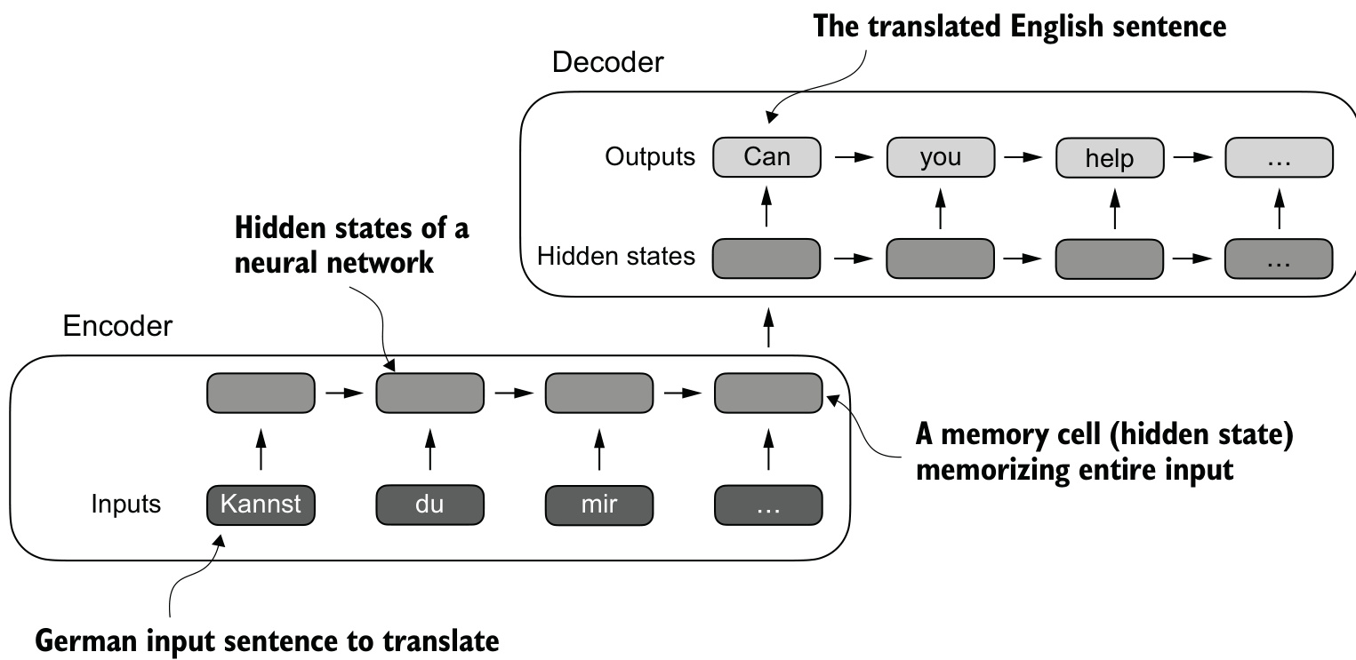
The encoder compresses the input into one hidden state; the decoder generates from it.

Raschka states the limitation plainly: the RNN cannot directly access earlier hidden states from the encoder during decoding. It relies solely on the current hidden state, which is supposed to encapsulate everything. On complex sentences with long-range dependencies, context is lost. You do not need to know how RNNs work internally — only this shortcoming, because it is what motivated attention.

Bahdanau attention, then self-attention

• 2014 — Bahdanau attention lets an RNN decoder selectively access all input positions at each decoding step. The single-vector bottleneck disappears.
• 2017 — researchers found RNNs are not required at all: the transformer, built entirely on self-attention.

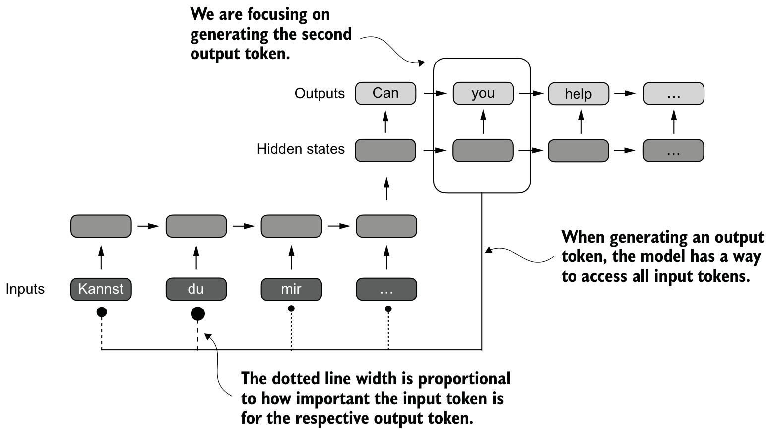
The decoder can access all input tokens selectively, weighted by attention.

Self-attention, defined

Self-attention lets each position in a sequence consider the relevance of — “attend to” — every other position in the same sequence.

The word “self” marks the contrast: ordinary attention relates elements of two different sequences (e.g. input and output); self-attention relates positions within one.

Simplified self-attention

The goal: a context vector

• Compute a context vector \(z^{(i)}\) for every input \(x^{(i)}\).
• \(z^{(i)}\) is an enriched embedding: it carries information about \(x^{(i)}\) and every other input.
• No trainable weights yet — the point is to isolate the shape of the computation.

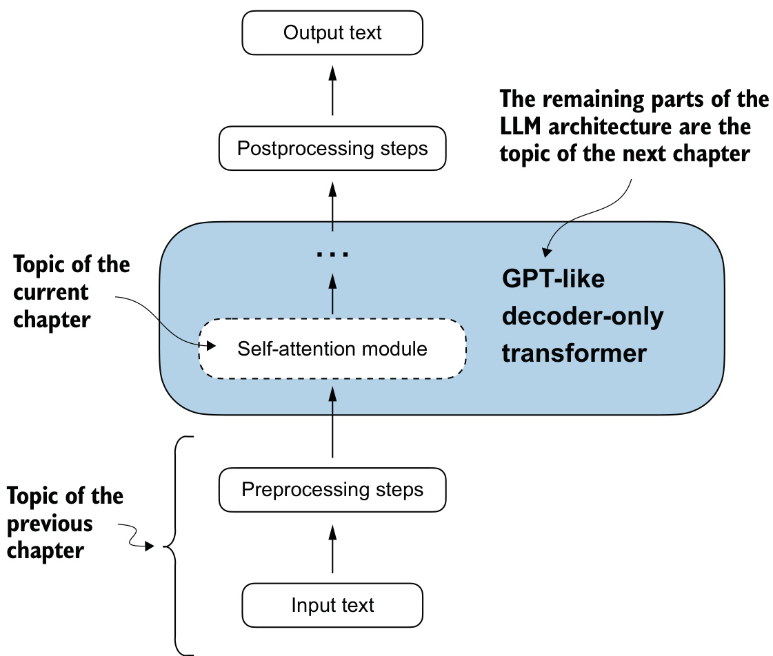
Each position interacts with and weighs the importance of every other position.

Step 1 — attention scores

For a query token \(x^{(q)}\) in a sequence of \(T\) tokens:

\[ \omega_{q,i} = x^{(q)} \cdot x^{(i)}, \qquad i = 1, \dots, T. \]

The dot product measures similarity: the higher it is, the more aligned two vectors are.

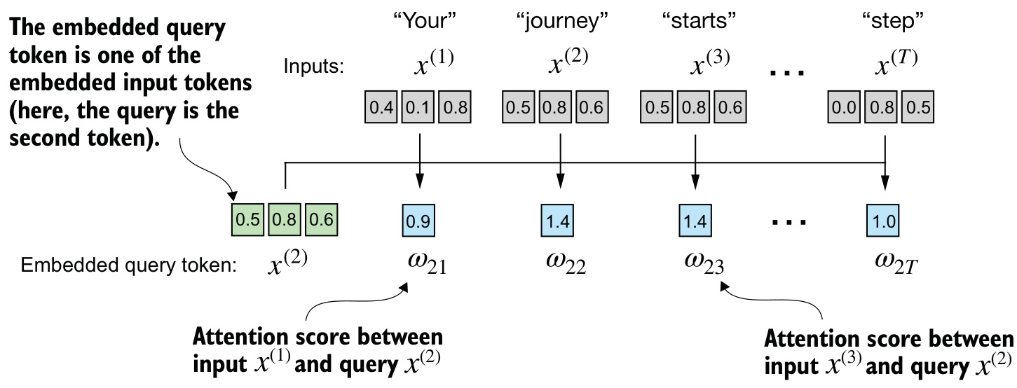
Attention scores \(\omega\) between the query and every input, computed as dot products.

Step 2 — attention weights

Normalize the scores so they sum to \(1\), using softmax:

\[ \alpha_{q,i} = \operatorname{softmax}(\omega_{q,\cdot})_i = \frac{e^{\omega_{q,i}}}{\sum_j e^{\omega_{q,j}}}. \]

Softmax is preferred over dividing by the sum: it handles extreme values better and has more favourable gradients, and it guarantees positive, interpretable weights.

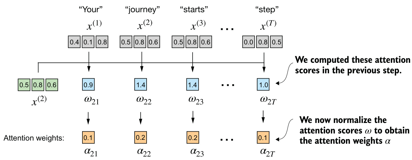
Normalizing the scores \(\omega_{2i}\) into weights \(\alpha_{2i}\).

Warn about numerical stability: a naive softmax — exponentiate, then divide — can overflow or underflow. Always use the framework’s stable implementation.

Step 3 — the context vector

\[ z^{(q)} = \sum_{i=1}^{T} \alpha_{q,i}\, x^{(i)}. \]

The context vector is the weighted sum of all input vectors, weighted by attention.

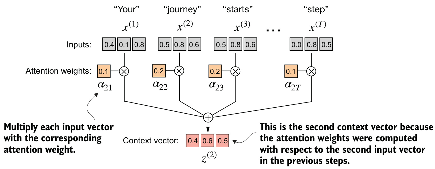
The context vector \(z^{(2)}\) combines all inputs, weighted by \(\alpha\).

All tokens at once

From one query to every query

Every token needs the same treatment as a query — not just one.

• A nested loop (outer over queries, inner over keys) is correct, but slow.
• It is only ever useful as a mental model of what the matrix form computes.

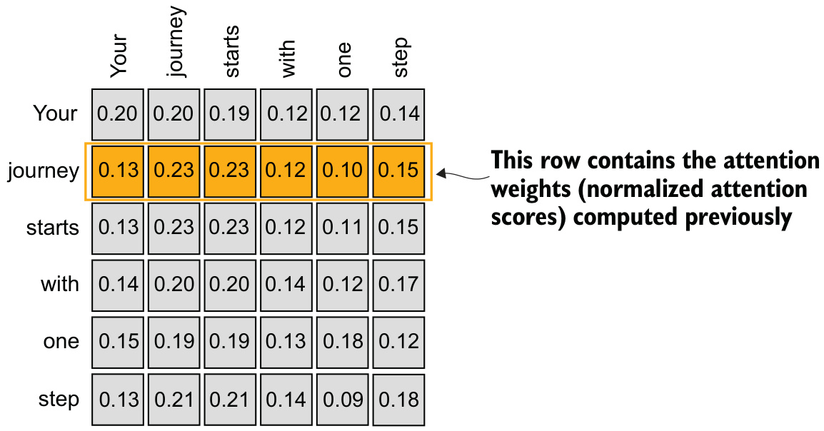
The second row’s weights, generalized to every row.

The matrix form

\[ \Omega = X X^{\top}, \qquad \Omega \in \mathbb{R}^{T \times T}, \]

where \(\Omega_{i,j}\) is the dot product of token \(i\) with token \(j\).

# pseudo-code — not literal syntax
scores = inputs @ inputs.transpose      # (T, T)
weights = softmax(scores, along=rows)   # each row sums to 1
context = weights @ inputs              # (T, d)

• One matrix multiplication replaces two nested loops.
• weights @ inputs gives one context vector per row.

Normalizing the right dimension

Softmax must run along the row — the axis over keys, for a fixed query.

Normalizing along the wrong axis is the classic bug here. Checking that every row sums to \(1\) is a cheap way to catch it.

\(\Omega \in \mathbb{R}^{T\times T} \;\to\; \alpha X \in \mathbb{R}^{T \times d}\)

Key ideas

• The full score matrix is \(XX^\top\), shape \(T \times T\).
• Softmax normalizes rows (over keys for a fixed query), not columns.
• The context-vector matrix \(\alpha X\) has shape \(T \times d\): one context vector per row.
• Matrix multiplication is not strictly required for correctness — it replaces nested loops with something equivalent, and far more efficient.

Trainable self-attention

Adding weights that learn

• So far the attention weights are fixed by the inputs — nothing is trained.
• The mechanism used in the original transformer, GPT, and most popular LLMs adds trainable weight matrices.
• Also called scaled dot-product attention.

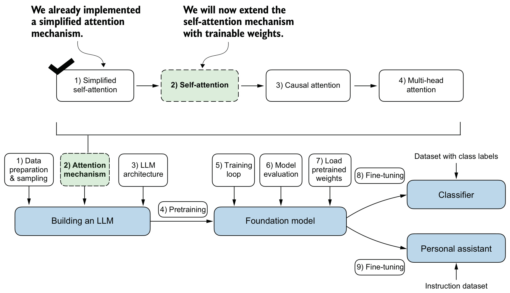
Adding trainable weights to the attention mechanism.

Three projections

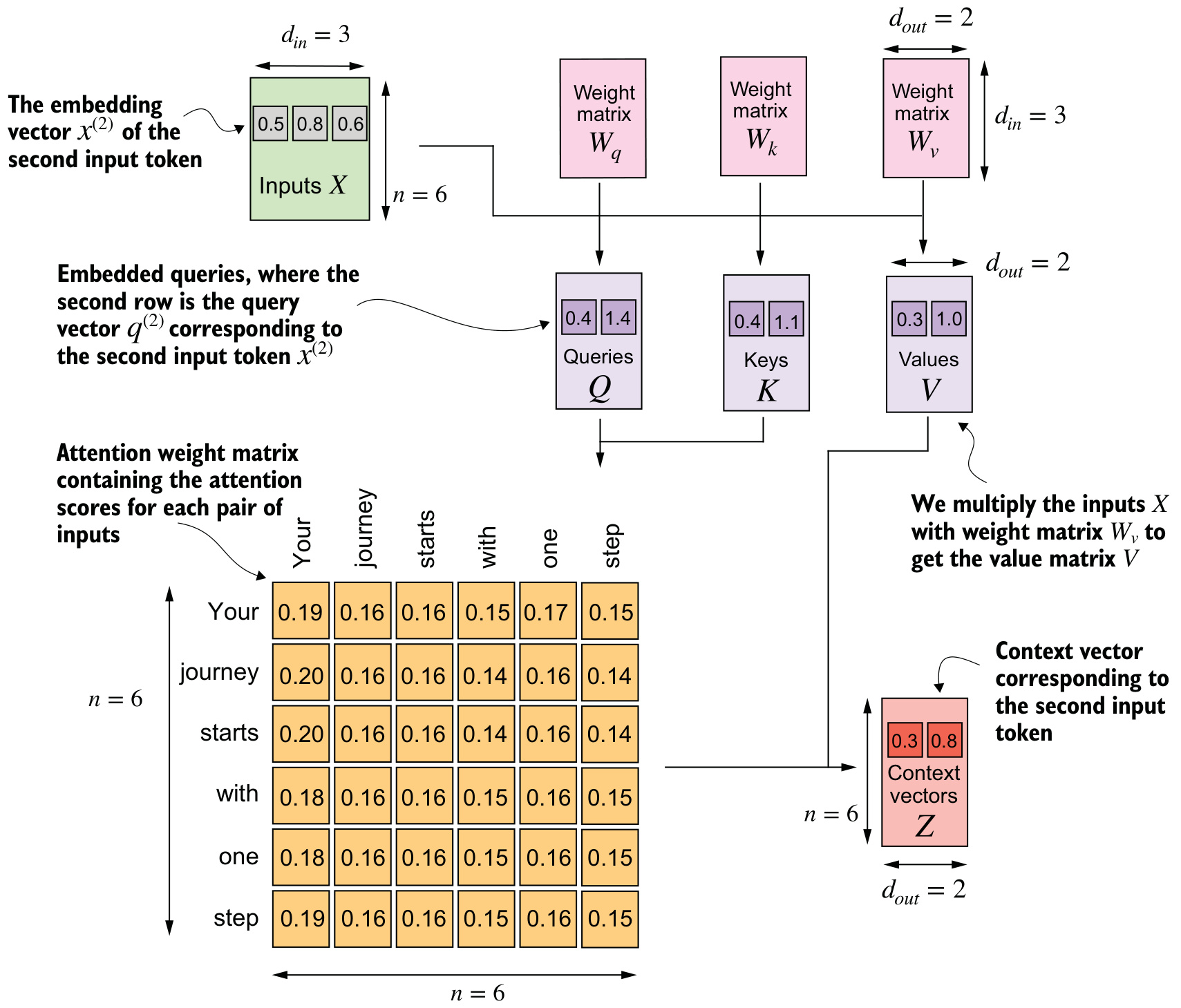
\[ q^{(i)} = W_q x^{(i)}, \qquad k^{(i)} = W_k x^{(i)}, \qquad v^{(i)} = W_v x^{(i)}. \]

Three trainable matrices \(W_q\), \(W_k\), \(W_v\) project each token into a query, key, and value vector.

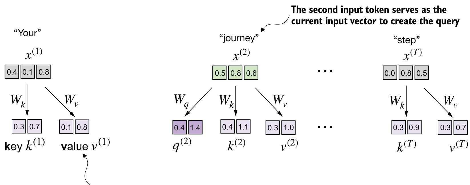
The query, key, and value vectors, each from its own weight matrix.

The terms come from information retrieval: a query is the search query — the item currently in focus. A key is the database index each item carries, used to match the query. A value is the content retrieved once the model decides which keys are relevant. Also flag: “weight” in W_q is a learned coefficient (weight parameter); an attention weight alpha is a dynamic, context-specific value computed on the fly. Same word, unrelated quantities.

Scores from queries and keys, scaled

\[ \omega_{q,i} = q^{(q)} \cdot k^{(i)}, \qquad \alpha_{q,\cdot} = \operatorname{softmax}\!\left(\frac{\omega_{q,\cdot}}{\sqrt{d_k}}\right). \]

• The score is again a dot product, now between transformed vectors.
• The scores are scaled by \(\sqrt{d_k}\) before the softmax — this is what gives the method its name.

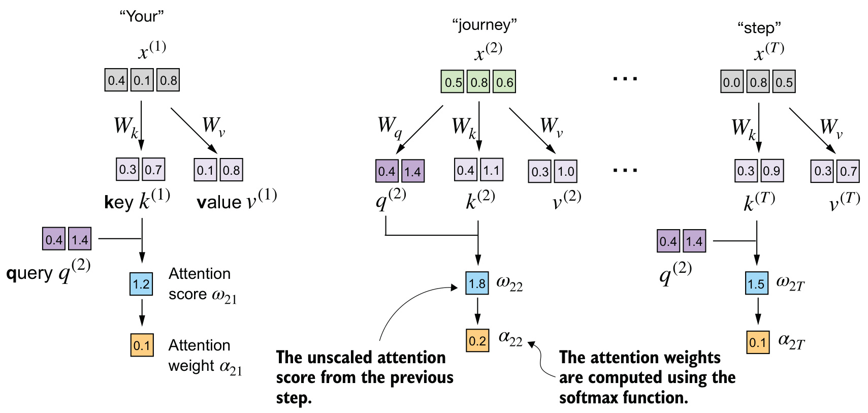
Scaled scores, normalized into attention weights.

Why scale: when the embedding dimension is scaled up — typically well over 1,000 for GPT-like LLMs — large dot products push softmax toward a step function, and gradients approach zero. Small gradients stall training. Dividing by sqrt(d_k) keeps the scores in a range where softmax still has useful gradients.

The context vector, from values

\[ z^{(q)} = \sum_i \alpha_{q,i}\, v^{(i)}. \]

The context vector is now a weighted sum over the value vectors, not the raw inputs.

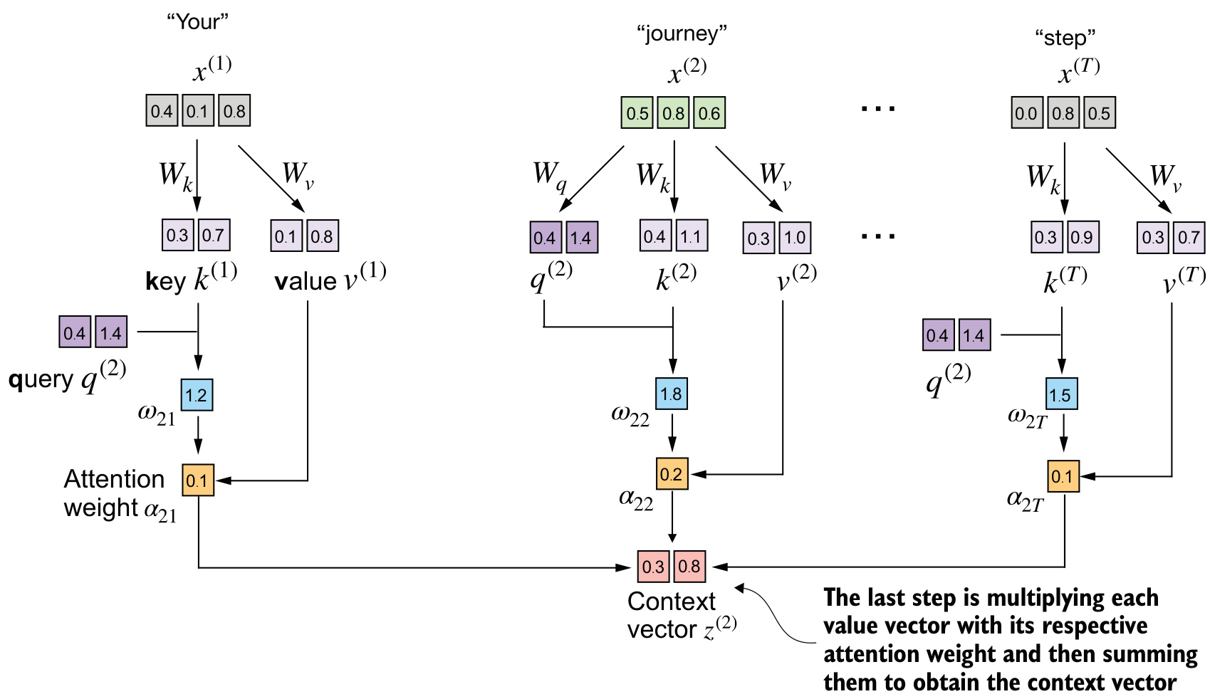
Combining the value vectors via the attention weights.

Packaging attention as a module

A reusable module

Given an input tensor, produce query, key, value projections, then run the same three steps as before.

# pseudo-code
class SelfAttention:
    def __init__(self, d_in, d_out):
        self.W_query, self.W_key, self.W_value = three trainable projections d_in -> d_out

    def forward(self, x):
        q, k, v = W_query(x), W_key(x), W_value(x)
        scores  = q @ k.T
        weights = softmax(scores / sqrt(d_out), along=rows)
        return weights @ v

Assembling the pieces

\(X\) is transformed by \(W_q, W_k, W_v\); the attention matrix comes from \(Q\) and \(K\); \(Z\) comes from the weights and \(V\).

Why a linear layer, not a raw matrix

A raw trainable parameter matrix and a bias-free linear layer compute the same operation.

A linear layer comes with an optimized weight initialization scheme, which contributes to more stable and effective training — this is why frameworks’ built-in linear layer is carried forward for the rest of the chapter.

Exercise 3.1 (Raschka): transfer the weight matrices from the linear-layer version into the raw-parameter version so both produce the same output, noting that a linear layer stores its weight matrix in transposed form. Point students to the textbook for the worked solution.

Causal masking

Restricting attention to the past

• Many LLM tasks require a token to consider only positions prior to it, when predicting the next token.
• Causal attention (masked attention) enforces this. Standard self-attention has no such restriction.

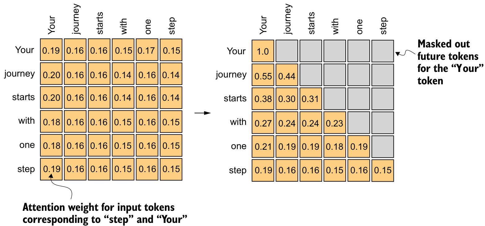
Weights above the diagonal are masked out.

Two equivalent routes

Zero, then renormalize. Compute ordinary weights, zero every entry above the diagonal, renormalize each row to sum to \(1\).

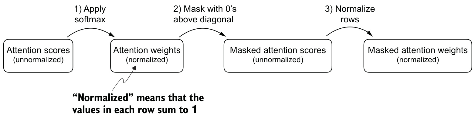
Softmax, then zero, then normalize.

Does this leak information? It might appear that masked tokens still influence the result, since their values entered the softmax denominator before masking. They do not — renormalizing after masking is equivalent to recomputing softmax over only the unmasked positions.

The efficient route

Fill with \(-\infty\) before the softmax. Since \(e^{-\infty} \to 0\), mask the scores directly, then apply softmax once.

No renormalization step is needed — each row already sums to \(1\).

Masking the scores with \(-\infty\) before softmax.

Both routes give the same lower-triangular attention matrix. The second is preferred: one softmax pass, not a softmax plus a separate normalization.

Dropout on attention

What dropout does

• Dropout randomly zeroes selected hidden-layer units during training.
• It prevents the model from over-relying on any specific set of units.
• Used only during training; disabled at inference.

In GPT-style transformers, dropout is applied right after the attention weights are computed — the more common of two possible placements.

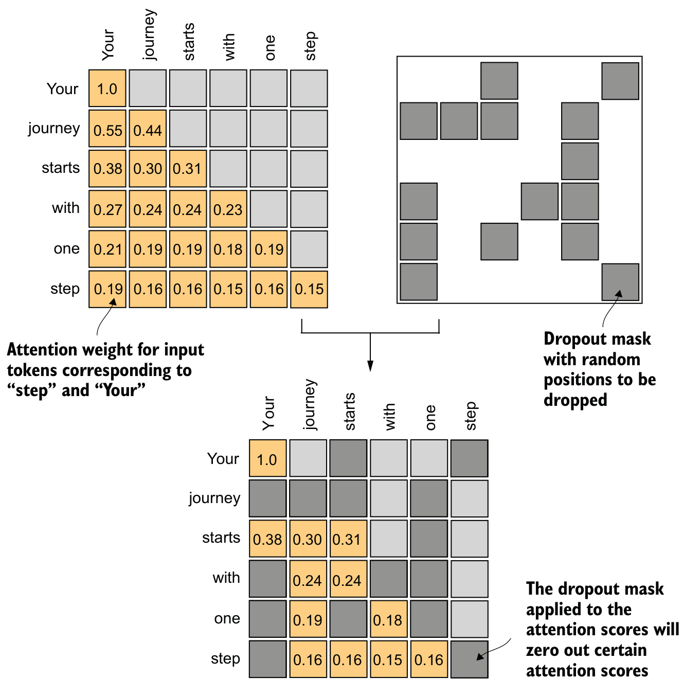
A dropout mask applied on top of the causal mask.

The rescaling

Dropout with rate \(p\) zeroes a random fraction \(p\) of entries, and scales every surviving entry by \(\dfrac{1}{1-p}\).

The scaling keeps the average influence of the attention mechanism consistent between training and inference, compensating for the reduced number of active elements.

Two visible consequences

• Rows no longer sum to \(1\) after the mask is applied.
• An entire row can occasionally be zeroed out.

Both are expected effects of the random mask, not errors.

Typical dropout rates used for attention are much lower than 0.5 — commonly 0.1 or 0.2. A higher rate is only illustrative for demonstrating the effect.

A batched causal attention module

From one sequence to a batch

Real inputs arrive as (batch, tokens, embedding dimension), because the data loader from the previous unit produces batched outputs.

The causal attention computation must run per example within the batch, not on a single sequence alone.

The module

# pseudo-code
class CausalAttention:
    def __init__(self, d_in, d_out, context_length, dropout):
        self.W_query, self.W_key, self.W_value = three projections d_in -> d_out
        self.dropout = dropout layer
        self.mask = upper-triangular mask, shape (context_length, context_length)

    def forward(self, x):                        # x: (batch, tokens, d_in)
        q, k, v = W_query(x), W_key(x), W_value(x)
        scores  = q @ k.transpose(last two dims)  # per-example, not global transpose
        scores  = fill(scores, mask, -inf)
        weights = softmax(scores / sqrt(d_out), along=rows)
        weights = dropout(weights)
        return weights @ v

Three details that matter

• Transpose only the last two axes. Leaves the batch axis untouched, so each example is handled independently.
• The mask is state, but not trainable state. Frameworks register it as a buffer so it moves with the model between devices automatically.
• The mask is sliced to the sequence length in use. Built once at the maximum context length; a shorter batch uses its top-left corner.

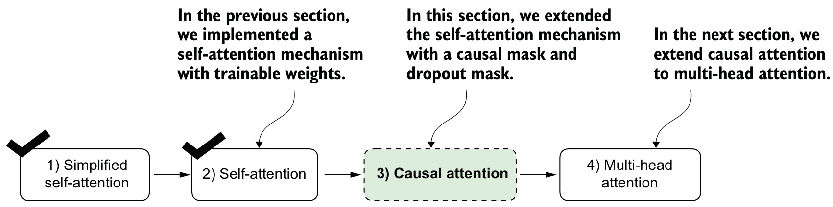
From simplified attention, to trainable weights, to a causal mask. Multi-head is next.

Multi-head by stacking

Several heads, run in parallel

Multi-head attention divides the mechanism into multiple heads, each operating independently, each with its own learned projections.

• A single causal attention module is single-head attention.
• Running several in parallel lets the model attend to different aspects of the data at once.

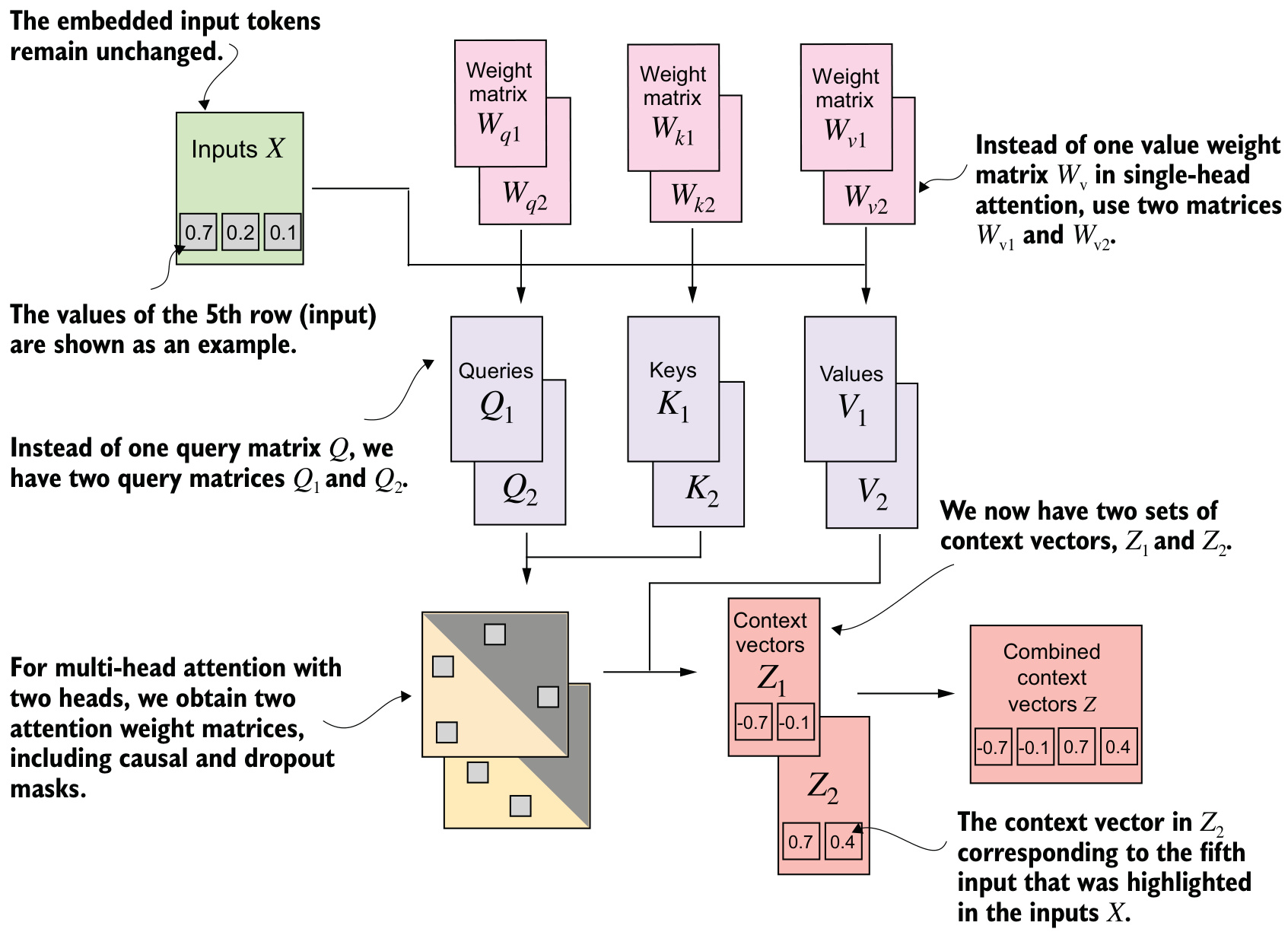
Two heads, two sets of \(W_q\), \(W_k\), \(W_v\); the two context-vector sets combine into one.

The direct implementation

The most direct implementation runs several independent copies of the single-head module and concatenates their outputs along the feature dimension.

• Each head owns its own \(W_q\), \(W_k\), \(W_v\).
• Output width is d_out * num_heads.

Where the cost is: running the heads one after another is not merely loop overhead — each head repeats the full projection matrix multiplication, one of the most expensive steps in the module. The next section removes that repetition.

Exercise 3.2 (Raschka): change the wrapper’s configuration, without modifying the class itself, so that with two heads the output context vectors end up two-dimensional rather than four-dimensional.

Multi-head by weight splitting

One projection, split internally

Rather than separate classes for a single head and a multi-head wrapper, combine them into one module.

• One larger projection per role — one \(W_q\), one \(W_k\), one \(W_v\).
• The result is split internally into individual heads by reshaping.

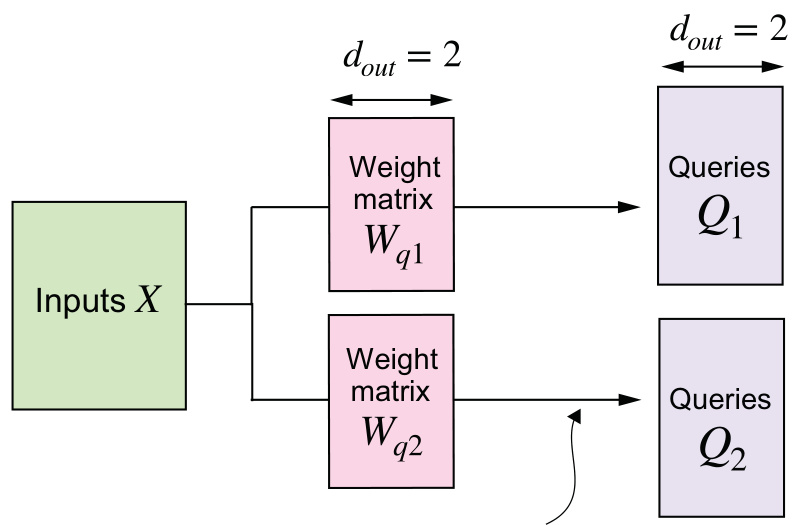
Two heads computed separately (top) vs. one larger projection split into heads (bottom).

The module

# pseudo-code
class MultiHeadAttention:
    def __init__(self, d_in, d_out, context_length, dropout, num_heads):
        assert d_out % num_heads == 0
        head_dim = d_out // num_heads
        self.W_query, self.W_key, self.W_value = three projections d_in -> d_out
        self.out_proj = projection d_out -> d_out
        self.mask = upper-triangular mask

    def forward(self, x):                            # x: (batch, tokens, d_in)
        q, k, v = W_query(x), W_key(x), W_value(x)    # (batch, tokens, d_out)
        split each of q, k, v into (batch, num_heads, tokens, head_dim)
        scores  = q @ k.transpose(last two dims)      # per head, batched
        scores  = fill(scores, mask, -inf)
        weights = dropout(softmax(scores / sqrt(head_dim), along=rows))
        context = weights @ v                         # per head
        recombine heads -> (batch, tokens, d_out)
        return out_proj(context)

Reading the reshapes

• Split. head_dim = d_out // num_heads — d_out must divide evenly across heads.
• Rearrange. The heads axis moves ahead of the tokens axis, so per-head matrices are contiguous.
• Batched attention. One batched matmul replaces one matmul per head.
• Recombine. Heads move back and flatten into the original d_out width.
• Output projection. A final linear layer, applied after recombining — not strictly necessary, but common in practice.

Batched matrix multiplication, checked by hand: the batched per-head multiplication is exactly equivalent to running the ordinary two-dimensional multiplication independently on each head’s slice — batching is a more compact and efficient way of expressing the same computation.

Why this version is used

Only one matrix multiplication per role is needed — one for keys, one for queries, one for values — regardless of the number of heads.

The stacked wrapper repeated that multiplication once per head. This version implements the identical mathematical operation, more efficiently.

For scale: the smallest GPT-2 model, 117M parameters, has 12 attention heads and embedding size 768. The largest, 1.5B parameters, has 25 heads and embedding size 1,600. In GPT models d_in and d_out are equal.

Exercise 3.3 (Raschka): configure this module to match the smallest GPT-2 model — 12 heads, embedding sizes of 768, context length of 1,024 tokens.

What to carry away

The shape of the mechanism

• Attention transforms inputs into context vectors that incorporate information about all inputs — what the RNN encoder-decoder bottleneck could not do.
• Self-attention computes a context vector as a weighted sum; in the simplified form, the weights come from dot products.
• Matrix multiplication is not strictly required for correctness — but \(XX^\top\) and \(\alpha X\) replace nested loops with the identical result, far more efficiently.

Trained, masked, and multiplied

• Scaled dot-product attention adds trainable \(W_q\), \(W_k\), \(W_v\) and divides the scores by \(\sqrt{d_k}\), keeping gradients from vanishing.
• A causal mask prevents access to future tokens; filling scores with \(-\infty\) before the softmax gets there in one pass, since each row still sums to \(1\).
• Multi-head attention runs several instances of causal attention; the efficient version obtains them from one projection per role, reshaped and batched.

Where next

Next: 4 Implementing a GPT model from scratch to generate text.

Attention is one sub-layer of a transformer block. The next unit adds the rest of the block, stacks the blocks into a full GPT architecture, and runs the loop that turns the model’s output into generated text.

For the full working implementation — tensor shapes, code for every step, worked numerical examples — point students to Raschka, Building a Large Language Model (from Scratch), chapter 3.