Lecture notes — 4 Implementing a GPT model from scratch to generate text
ver. 1.2.0, 4_implementing_a_gpt_model_from_scratch_to_generate_text
← 4 Implementing a GPT model from scratch to generate text
ver. 1.2.0 · 2026-09-02 16:27:46
Where this fits
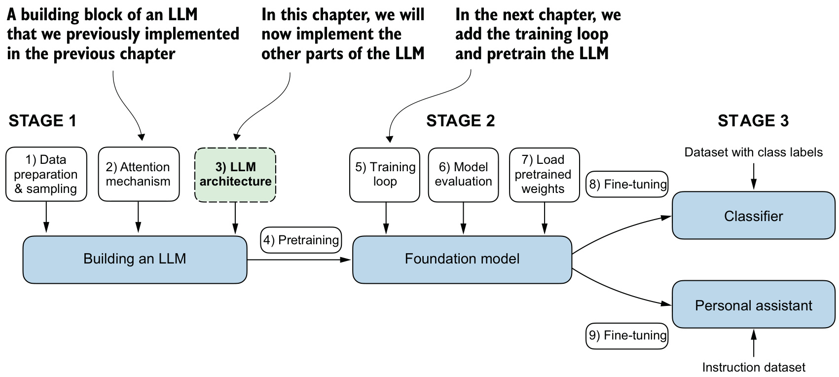
The previous unit, 3 Coding attention mechanisms, ended with a MultiHeadAttention module: scaled dot-product scores, a causal mask that sets future positions to \(-\infty\) before the softmax, dropout on the attention weights, and heads parallelized by reshaping a single set of projections. That module is one sub-layer of one block of a GPT model.
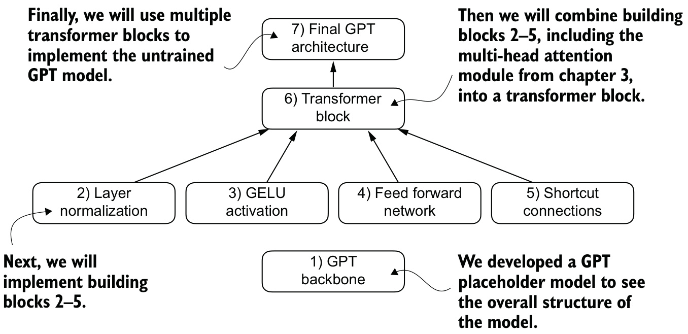
This unit supplies the remainder. Layer normalization, the GELU activation, a position-wise feed-forward network and residual shortcut connections are implemented as separate PyTorch modules, composed with masked multi-head attention into a TransformerBlock, and stacked twelve deep inside a GPTModel matching the GPT-2 124 million parameter configuration. The finished model is measured — parameter count and memory footprint — and then run in an autoregressive loop that produces text.
No weight is trained here. Building a Large Language Model (from scratch), Sebastian Raschka, 2024, Manning Books places this work as step 3 of stage 1 in the construction of an LLM: the architecture is written before the training loop exists.
Learning outcomes
gpt-configuration-and-skeleton— Specify a GPT-2 124M configuration and build a placeholder model that carries tensors end to end.layer-normalization— Implement a LayerNorm module with learnable scale and shift.gelu-and-feed-forward— Implement GELU and the position-wise feed-forward sub-network.shortcut-connections— Use residual shortcut connections to keep gradients flowing through deep stacks.transformer-block— Compose attention, feed-forward, pre-LayerNorm, dropout and shortcuts into one TransformerBlock.assembling-the-gpt-model— Assemble the full GPTModel from embeddings, a block stack, a final norm and an output head.parameter-count-and-memory— Compute a model’s parameter count, memory footprint and the effect of weight tying.autoregressive-greedy-generation— Write the autoregressive loop that turns logits into generated text.
Concepts introduced
- GPT architecture — a decoder-only transformer that generates text one token at a time, built from token and positional embeddings, a stack of identical transformer blocks, a final layer normalization and a linear projection to the vocabulary.
- Layer normalization — normalization of a layer’s activations to mean \(0\) and variance \(1\) along the feature dimension, followed by a learnable scale and shift.
- GELU activation — \(\text{GELU}(x) = x \cdot \Phi(x)\), where \(\Phi\) is the cumulative distribution function of the standard normal distribution; smooth everywhere, and nonzero for most negative inputs.
- Feed-forward network — two linear layers with a GELU between them, expanding the embedding dimension by a factor of four and contracting it back, applied to each token position independently.
- Shortcut connections — the addition of a layer’s input to its output, \(x_{l+1} = x_l + F(x_l)\), giving the gradient a path that bypasses the layer.
- Transformer block — masked multi-head attention and a feed-forward network, each preceded by layer normalization and followed by dropout, each wrapped in a shortcut.
- Weight tying — sharing one \(50257 \times 768\) weight matrix between the token embedding layer and the output projection.
- Greedy decoding — selecting, at each generation step, the token whose predicted probability is largest.
Configuration and a dummy architecture
A GPT model is a large deep neural network designed to generate text one word, or token, at a time. Its architecture is not proportionally complicated, because most of its components are repeated. The specific target here is the smallest version of GPT-2, with 124 million parameters, described in “Language Models Are Unsupervised Multitask Learners” by Radford et al. The original report states 117 million parameters; that figure was later corrected to 124 million.
A parameter is a trainable weight of the model — an internal variable adjusted during training to minimize a loss function. A layer represented by a \(2{,}048 \times 2{,}048\) matrix of weights therefore holds \(2{,}048 \times 2{,}048 = 4{,}194{,}304\) parameters.
The configuration
Every module written below reads its shape from one dictionary.
GPT_CONFIG_124M = {
    "vocab_size": 50257,    # Vocabulary size
    "context_length": 1024, # Context length
    "emb_dim": 768,         # Embedding dimension
    "n_heads": 12,          # Number of attention heads
    "n_layers": 12,         # Number of layers
    "drop_rate": 0.1,       # Dropout rate
    "qkv_bias": False       # Query-Key-Value bias
}vocab_sizeis the 50,257 words of the BPE tokenizer of the tokenization unit.context_lengthis the maximum number of input tokens the model can handle, through its positional embeddings.emb_dimtransforms each token into a 768-dimensional vector.n_headsis the count of attention heads in the multi-head attention mechanism.n_layersis the number of transformer blocks.drop_rateof \(0.1\) implies a 10% random drop out of hidden units, to prevent overfitting.qkv_biasdetermines whether theLinearlayers of multi-head attention include a bias vector for the query, key and value computations. It is disabled here, following the norms of modern LLMs.
The skeleton
DummyGPTModel fixes the data path before any real component exists. Its transformer block and its layer normalization return their input unchanged.
import torch
import torch.nn as nn

class DummyGPTModel(nn.Module):
    def __init__(self, cfg):
        super().__init__()
        self.tok_emb = nn.Embedding(cfg["vocab_size"], cfg["emb_dim"])
        self.pos_emb = nn.Embedding(cfg["context_length"], cfg["emb_dim"])
        self.drop_emb = nn.Dropout(cfg["drop_rate"])
        self.trf_blocks = nn.Sequential(
            *[DummyTransformerBlock(cfg)
              for _ in range(cfg["n_layers"])]
        )
        self.final_norm = DummyLayerNorm(cfg["emb_dim"])
        self.out_head = nn.Linear(
            cfg["emb_dim"], cfg["vocab_size"], bias=False
        )

    def forward(self, in_idx):
        batch_size, seq_len = in_idx.shape
        tok_embeds = self.tok_emb(in_idx)
        pos_embeds = self.pos_emb(
            torch.arange(seq_len, device=in_idx.device)
        )
        x = tok_embeds + pos_embeds
        x = self.drop_emb(x)
        x = self.trf_blocks(x)
        x = self.final_norm(x)
        logits = self.out_head(x)
        return logits

class DummyTransformerBlock(nn.Module):
    def __init__(self, cfg):
        super().__init__()

    def forward(self, x):
        return x

class DummyLayerNorm(nn.Module):
    def __init__(self, normalized_shape, eps=1e-5):
        super().__init__()

    def forward(self, x):
        return x
A batch of two four-token texts is tokenized with the gpt2 encoding.
import tiktoken

tokenizer = tiktoken.get_encoding("gpt2")
batch = []
txt1 = "Every effort moves you"
txt2 = "Every day holds a"

batch.append(torch.tensor(tokenizer.encode(txt1)))
batch.append(torch.tensor(tokenizer.encode(txt2)))
batch = torch.stack(batch, dim=0)
print(batch)
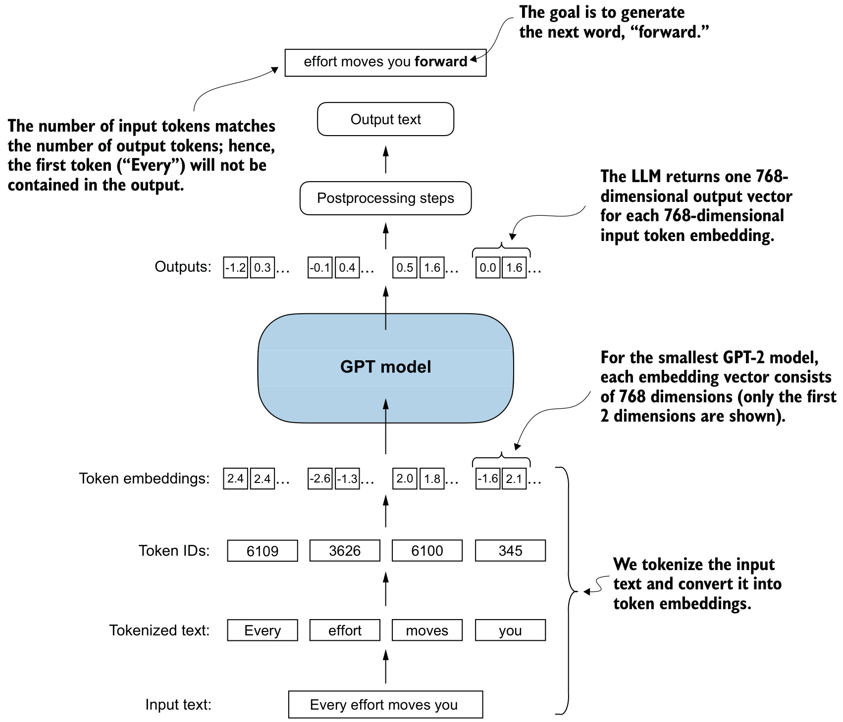
The resulting token IDs are tensor([[6109, 3626, 6100, 345], [6109, 1110, 6622, 257]]). Feeding them through the placeholder model returns Output shape: torch.Size([2, 4, 50257]). Each of the eight token positions has one unnormalized score per vocabulary entry. Those scores are called logits. The 50,257 dimensions exist because each dimension refers to one unique token of the vocabulary; postprocessing code converts such a vector back into a token ID, and the ID back into a word.
GPT-3 is fundamentally the same architecture, scaled from GPT-2’s 1.5 billion parameters to 175 billion and trained on more data. According to Lambda Labs, training GPT-3 would take 355 years on a single V100 datacenter GPU and 665 years on a consumer RTX 8000 GPU. GPT-2 can be run on a single laptop.
Learning outcomes
- gpt-configuration-and-skeleton Specify a GPT-2 124M configuration and build a placeholder model that carries tensors end to end.
Concepts
- gpt-architecture the whole model is fixed by seven entries of a configuration dictionary and a data path from token IDs to logits
- transformer-block a pass-through placeholder occupies the block’s position while the data path is verified
- layer-normalization a placeholder mimicking the interface stands in the final normalization slot
Layer normalization
Training deep neural networks with many layers can prove challenging because of vanishing or exploding gradients. Such problems lead to unstable training dynamics, and the search for weights that minimize the loss function struggles.
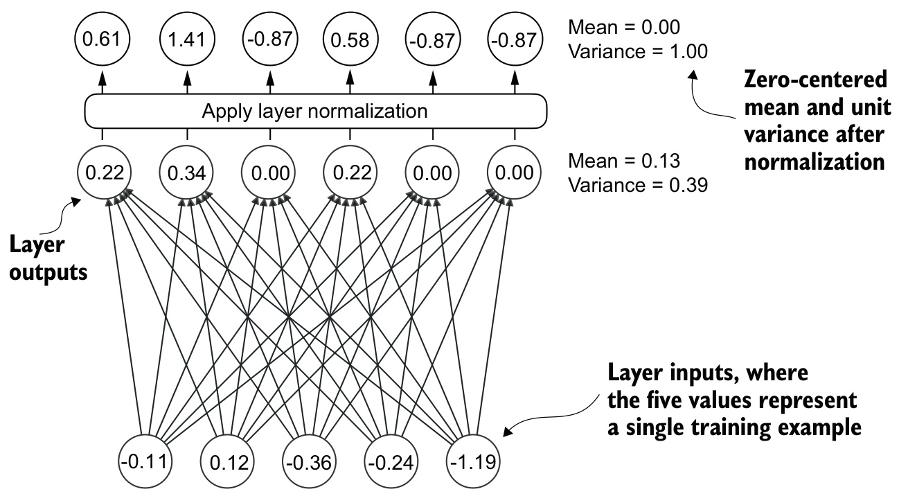
Layer normalization adjusts the activations of a layer to have a mean of \(0\) and a variance of \(1\), also known as unit variance. It operates on the last dimension of the tensor, which is the embedding dimension. For a tensor of shape [batch_size, num_tokens, embedding_size], dim=-1 normalizes across the feature dimension without any change of index. This is unlike batch normalization, which normalizes across the batch dimension; because layer normalization treats each input independently of the batch size, it offers more flexibility in distributed training and in resource-constrained deployment.
The operation, step by step
A layer of five inputs and six outputs, applied to two examples:
torch.manual_seed(123)
batch_example = torch.randn(2, 5)
layer = nn.Sequential(nn.Linear(5, 6), nn.ReLU())
out = layer(batch_example)
print(out)
The output contains no negative values, because ReLU thresholds negative inputs to \(0\):
tensor([[0.2260, 0.3470, 0.0000, 0.2216, 0.0000, 0.0000],
        [0.2133, 0.2394, 0.0000, 0.5198, 0.3297, 0.0000]],
       grad_fn=<ReluBackward0>)
The mean and variance of each row are taken with keepdim=True, which preserves the number of dimensions of the input; without it the mean of a \(2 \times 6\) tensor would be the vector [0.1324, 0.2170] rather than the \(2 \times 1\) matrix [[0.1324], [0.2170]].
mean = out.mean(dim=-1, keepdim=True)
var = out.var(dim=-1, keepdim=True)
That gives means \(0.1324\) and \(0.2170\), variances \(0.0231\) and \(0.0398\). Subtracting the mean and dividing by the square root of the variance,
\[\hat{x} = \frac{x - \mu}{\sqrt{\sigma^2}},\]
produces out_norm = (out - mean) / torch.sqrt(var) with means \(-5.9605 \times 10^{-8}\) and \(1.9868 \times 10^{-8}\) and variances of exactly \(1\). The first value is \(-0.000000059605\), not \(0\), because of the finite precision with which computers represent numbers.
The module
class LayerNorm(nn.Module):
    def __init__(self, emb_dim):
        super().__init__()
        self.eps = 1e-5
        self.scale = nn.Parameter(torch.ones(emb_dim))
        self.shift = nn.Parameter(torch.zeros(emb_dim))

    def forward(self, x):
        mean = x.mean(dim=-1, keepdim=True)
        var = x.var(dim=-1, keepdim=True, unbiased=False)
        norm_x = (x - mean) / torch.sqrt(var + self.eps)
        return self.scale * norm_x + self.shift
eps is a small constant added to the variance to prevent division by zero. scale and shift are trainable parameters of the same dimension as the input, which the LLM adjusts during training if doing so improves performance on the training task. Instantiated with LayerNorm(emb_dim=6) and applied to out, the module returns means of \(-0.0000\) and \(0.0000\) and variances of \(0.9995\) and \(0.9997\).
unbiased=False divides by the number of inputs \(n\) rather than applying Bessel’s correction, which uses \(n - 1\). The result is the biased estimate of the variance. For LLMs, where the embedding dimension \(n\) is significantly large, the difference between \(n\) and \(n-1\) is practically negligible. The setting was chosen for compatibility with GPT-2’s normalization layers and because it reflects TensorFlow’s default behavior, which was used to implement the original GPT-2 model — pretrained weights load correctly as a result.
In GPT-2 and modern transformer architectures, layer normalization is applied before the multi-head attention module and before the final output layer.
Learning outcomes
- layer-normalization Implement a LayerNorm module with learnable scale and shift.
Concepts
- layer-normalization standardizing each token’s activation vector to zero mean and unit variance, then scaling and shifting it by trained vectors, stabilizes optimization
GELU and the feed-forward network
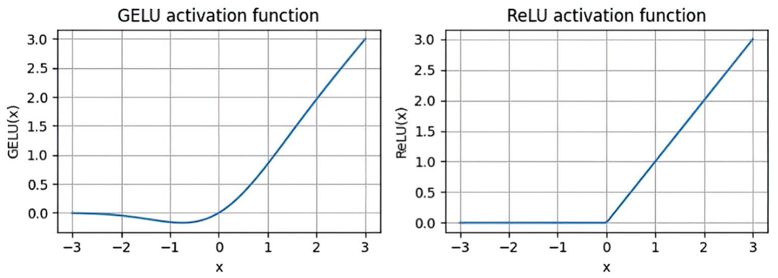
Historically the ReLU activation function has been commonly used in deep learning. In LLMs, other activation functions are employed, among them GELU, the Gaussian error linear unit, and SwiGLU, the Swish-gated linear unit. Both are smooth and incorporate Gaussian and sigmoid-gated linear units respectively.
The exact definition of the GELU activation is \(\text{GELU}(x) = x \cdot \Phi(x)\), where \(\Phi(x)\) is the cumulative distribution function of the standard Gaussian distribution. In practice a computationally cheaper approximation is used, found by curve fitting, with which the original GPT-2 model was also trained:
\[GELU(x) \approx 0.5 \cdot x \cdot \left(1 + tanh\left[\sqrt{\frac{2}{\pi}} \cdot \left(x + 0.044715 \cdot x^3\right)\right]\right)\]
class GELU(nn.Module):
    def __init__(self):
        super().__init__()

    def forward(self, x):
        return 0.5 * x * (1 + torch.tanh(
            torch.sqrt(torch.tensor(2.0 / torch.pi)) *
            (x + 0.044715 * torch.pow(x, 3))
        ))
Plotted over \(100\) points on \([-3, 3]\), ReLU is a piecewise linear function that outputs the input directly if it is positive and zero otherwise. GELU is a smooth, nonlinear function that approximates ReLU but with a nonzero gradient for almost all negative values, the exception being approximately \(x = -0.75\). Two consequences follow. The smoothness allows more nuanced adjustments to the model’s parameters during training, where ReLU’s sharp corner at zero can make optimization harder in very deep or complex architectures. And because GELU allows a small, nonzero output for negative values, neurons that receive negative input can still contribute to the learning process, albeit to a lesser extent than positive inputs.
The module
class FeedForward(nn.Module):
    def __init__(self, cfg):
        super().__init__()
        self.layers = nn.Sequential(
            nn.Linear(cfg["emb_dim"], 4 * cfg["emb_dim"]),
            GELU(),
            nn.Linear(4 * cfg["emb_dim"], cfg["emb_dim"]),
        )

    def forward(self, x):
        return self.layers(x)
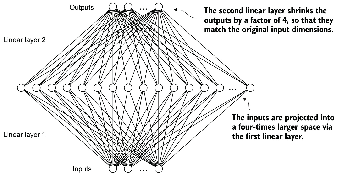
The feed-forward network is a small neural network of two Linear layers and one GELU activation. With GPT_CONFIG_124M["emb_dim"] = 768, the first linear layer increases the embedding dimension by a factor of \(4\), from \(768\) to \(3072\); the second decreases it by a factor of \(4\), back to \(768\). Applied to x = torch.rand(2, 3, 768), the module returns torch.Size([2, 3, 768]).
The expansion into a higher-dimensional space, the nonlinear GELU, and the contraction back allow the exploration of a richer representation space.
Input and output dimensions are identical, and the internal width is where the additional capacity sits.
The embedding size per token is fixed when the weights are initialized, while the batch size and the number of tokens may vary.
The same weights are applied at every token position, independently. No information moves between positions inside this module.
Uniform input and output dimensions permit multiple such layers to be stacked without adjusting dimensions between them.
That uniformity is what makes the transformer block repeatable.
Learning outcomes
- gelu-and-feed-forward Implement GELU and the position-wise feed-forward sub-network.
Concepts
- gelu-activation the tanh approximation of \(x \cdot \Phi(x)\) keeps a nonzero gradient for almost all negative inputs, unlike ReLU’s hard zero
- feed-forward-network two linear layers around a GELU expand each token’s 768 features to 3,072 and project them back
Shortcut connections and gradient flow
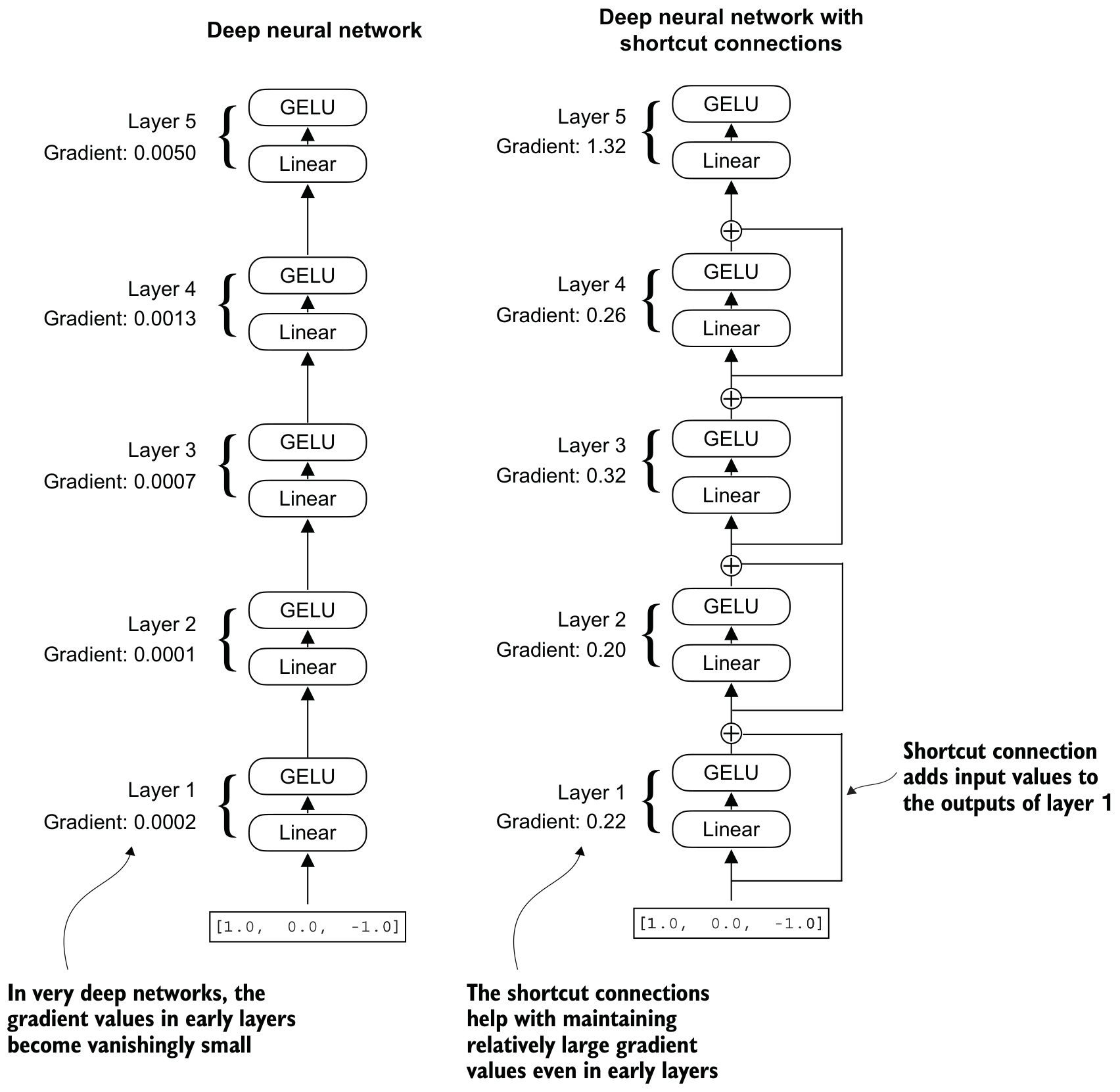
Shortcut connections, also known as skip or residual connections, were originally proposed for deep networks in computer vision, specifically in residual networks, to mitigate the challenge of vanishing gradients. The vanishing gradient problem is the issue where gradients, which guide weight updates during training, become progressively smaller as they propagate backward through the layers, making it difficult to train earlier layers effectively. A shortcut connection creates an alternative, shorter path for the gradient by adding the output of one layer to the output of a later layer.
class ExampleDeepNeuralNetwork(nn.Module):
    def __init__(self, layer_sizes, use_shortcut):
        super().__init__()
        self.use_shortcut = use_shortcut
        self.layers = nn.ModuleList([
            nn.Sequential(nn.Linear(layer_sizes[0], layer_sizes[1]),
                          GELU()),
            nn.Sequential(nn.Linear(layer_sizes[1], layer_sizes[2]),
                          GELU()),
            nn.Sequential(nn.Linear(layer_sizes[2], layer_sizes[3]),
                          GELU()),
            nn.Sequential(nn.Linear(layer_sizes[3], layer_sizes[4]),
                          GELU()),
            nn.Sequential(nn.Linear(layer_sizes[4], layer_sizes[5]),
                          GELU())
        ])

    def forward(self, x):
        for layer in self.layers:
            layer_output = layer(x)
            if self.use_shortcut and x.shape == layer_output.shape:
                x = x + layer_output
            else:
                x = layer_output
        return x
The shortcut is applied only when x.shape == layer_output.shape. An addition between tensors of different shapes is not defined, so the last layer of this network, which maps three values to one, takes the plain path.
Measuring the gradients
Five layers accept three input values and return three, except the last, which returns a single output value.
layer_sizes = [3, 3, 3, 3, 3, 1]
sample_input = torch.tensor([[1., 0., -1.]])
torch.manual_seed(123)
model_without_shortcut = ExampleDeepNeuralNetwork(
    layer_sizes, use_shortcut=False
)
def print_gradients(model, x):
output = model(x)
target = torch.tensor([[0.]])
loss = nn.MSELoss()
loss = loss(output, target)
loss.backward()
for name, param in model.named_parameters():
if 'weight' in name:
print(f"{name} has gradient mean of {param.grad.abs().mean().item()}")The loss measures how close the model output is to a target, here the value \(0\). loss.backward() computes the gradient of the loss with respect to each weight. For a \(3 \times 3\) weight matrix, the mean absolute value of its nine gradients is printed, so that layers can be compared by a single number.
Without shortcuts, print_gradients(model_without_shortcut, sample_input) gives
layers.0.0.weight has gradient mean of 0.00020173587836325169
layers.1.0.weight has gradient mean of 0.0001201116101583466
layers.2.0.weight has gradient mean of 0.0007152041653171182
layers.3.0.weight has gradient mean of 0.001398873864673078
layers.4.0.weight has gradient mean of 0.005049646366387606
The gradients become smaller from the last layer, layers.4, to the first, layers.0 — a factor of about \(25\) across five layers. With use_shortcut=True and the same seed,
layers.0.0.weight has gradient mean of 0.22169792652130127
layers.1.0.weight has gradient mean of 0.20694105327129364
layers.2.0.weight has gradient mean of 0.32896995544433594
layers.3.0.weight has gradient mean of 0.2665732502937317
layers.4.0.weight has gradient mean of 1.3258541822433472
The last layer still carries a larger gradient than the others, but the value stabilizes toward the first layer instead of shrinking to a vanishingly small value.
Learning outcomes
- shortcut-connections Use residual shortcut connections to keep gradients flowing through deep stacks.
Concepts
- shortcut-connections adding a layer’s input to its output raises the first layer’s mean absolute gradient from \(0.0002\) to \(0.2217\) in a five-layer network
The transformer block
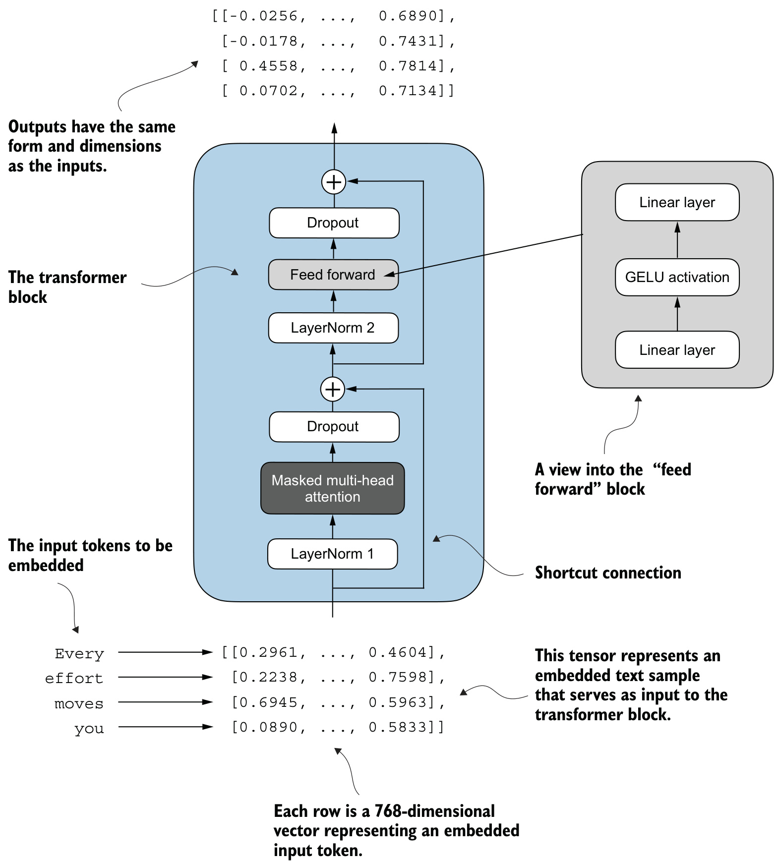
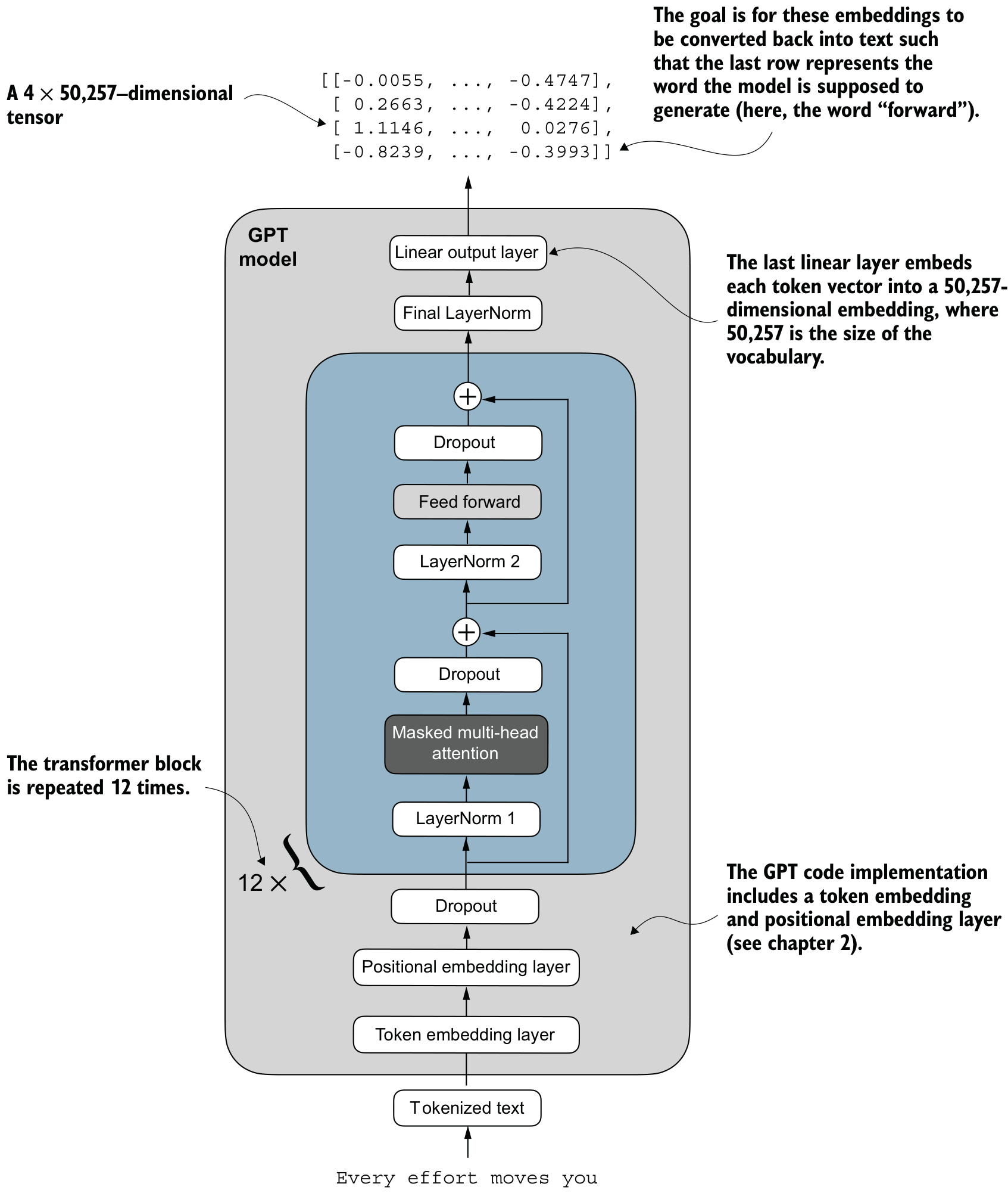
The transformer block is repeated a dozen times in the 124-million-parameter GPT-2 architecture. It combines multi-head attention, layer normalization, dropout, feed forward layers and GELU activations.
from chapter03 import MultiHeadAttention

class TransformerBlock(nn.Module):
    def __init__(self, cfg):
        super().__init__()
        self.att = MultiHeadAttention(
            d_in=cfg["emb_dim"],
            d_out=cfg["emb_dim"],
            context_length=cfg["context_length"],
            num_heads=cfg["n_heads"],
            dropout=cfg["drop_rate"],
            qkv_bias=cfg["qkv_bias"])
        self.ff = FeedForward(cfg)
        self.norm1 = LayerNorm(cfg["emb_dim"])
        self.norm2 = LayerNorm(cfg["emb_dim"])
        self.drop_shortcut = nn.Dropout(cfg["drop_rate"])

    def forward(self, x):
        shortcut = x
        x = self.norm1(x)
        x = self.att(x)
        x = self.drop_shortcut(x)
        x = x + shortcut

        shortcut = x
        x = self.norm2(x)
        x = self.ff(x)
        x = self.drop_shortcut(x)
        x = x + shortcut
        return x
Both sub-layers follow the same four steps: save the input as shortcut, normalize, apply the operation, apply dropout, and add the original input back.
Layer normalization is applied before each of the two components, and dropout after them to regularize the model and prevent overfitting. This arrangement is known as Pre-LayerNorm. Older architectures, such as the original transformer model, applied layer normalization after the self-attention and feed forward networks instead, known as Post-LayerNorm, which often leads to worse training dynamics.
The two sub-layers do different work. The self-attention mechanism in the multi-head attention block identifies and analyzes relationships between elements in the input sequence. The feed forward network modifies the data individually at each position. The combination enables a more nuanced understanding of the input and enhances the model’s overall capacity for handling complex data patterns.
Shape preservation
torch.manual_seed(123)
x = torch.rand(2, 4, 768)
block = TransformerBlock(GPT_CONFIG_124M)
output = block(x)

print("Input shape:", x.shape)
print("Output shape:", output.shape)
Both print torch.Size([2, 4, 768]). The preservation of shape throughout the transformer block architecture is not incidental but a crucial aspect of its design. Each output vector corresponds directly to an input vector, maintaining a one-to-one relationship. The content, however, is not preserved: the output is a context vector that encapsulates information from the entire input sequence. The physical dimensions of the sequence remain unchanged as it passes through the block, while each output vector is re-encoded to integrate contextual information from across the input sequence.
Learning outcomes
- transformer-block Compose attention, feed-forward, pre-LayerNorm, dropout and shortcuts into one TransformerBlock.
- layer-normalization Implement a LayerNorm module with learnable scale and shift.
- shortcut-connections Use residual shortcut connections to keep gradients flowing through deep stacks.
Concepts
- transformer-block two residual sub-layers, attention then feed-forward, that leave the tensor shape \([B, T, 768]\) unchanged
- layer-normalization a separate
LayerNormprecedes each sub-layer, the Pre-LayerNorm arrangement of GPT-2 - feed-forward-network the second sub-layer transforms each token position on its own, after attention has mixed across positions
- shortcut-connections each sub-layer’s input is added back to its output, so the block’s two additions give the gradient a direct path
Assembling the GPT model
The two placeholders of the skeleton, DummyTransformerBlock and DummyLayerNorm, are replaced by TransformerBlock and LayerNorm. The transformer block is repeated 12 times, as specified by the n_layers entry of GPT_CONFIG_124M; in the largest GPT-2 model, with 1,542 million parameters, it is repeated 48 times.
class GPTModel(nn.Module):
    def __init__(self, cfg):
        super().__init__()
        self.tok_emb = nn.Embedding(cfg["vocab_size"], cfg["emb_dim"])
        self.pos_emb = nn.Embedding(cfg["context_length"], cfg["emb_dim"])
        self.drop_emb = nn.Dropout(cfg["drop_rate"])

        self.trf_blocks = nn.Sequential(
            *[TransformerBlock(cfg) for _ in range(cfg["n_layers"])])

        self.final_norm = LayerNorm(cfg["emb_dim"])
        self.out_head = nn.Linear(
            cfg["emb_dim"], cfg["vocab_size"], bias=False
        )

    def forward(self, in_idx):
        batch_size, seq_len = in_idx.shape
        tok_embeds = self.tok_emb(in_idx)

        pos_embeds = self.pos_emb(
            torch.arange(seq_len, device=in_idx.device)
        )
        x = tok_embeds + pos_embeds
        x = self.drop_emb(x)
        x = self.trf_blocks(x)
        x = self.final_norm(x)
        logits = self.out_head(x)
        return logits
The embedding layers convert input token indices into dense vectors and add positional information.
torch.arange(seq_len, device=in_idx.device)builds the position indices on the same device as the input data, which allows the model to be trained on a CPU or a GPU depending on where the input sits.The output from the final transformer block passes through a final layer normalization before the linear output layer.
That normalization standardizes the outputs of the transformer blocks and stabilizes the learning process.
The output head is a linear layer without bias, projecting into the vocabulary space of the tokenizer.
It maps the transformer’s output to 50,257 dimensions, one per vocabulary entry, to predict the next token in the sequence.
Running the batch of two four-token texts through GPTModel(GPT_CONFIG_124M) gives Output shape: torch.Size([2, 4, 50257]) — the shape the dummy model produced, now computed by a working network. The forward method computes the logits, representing the next token’s unnormalized probabilities.
Learning outcomes
- assembling-the-gpt-model Assemble the full GPTModel from embeddings, a block stack, a final norm and an output head.
- transformer-block Compose attention, feed-forward, pre-LayerNorm, dropout and shortcuts into one TransformerBlock.
- gelu-and-feed-forward Implement GELU and the position-wise feed-forward sub-network.
Concepts
- gpt-architecture embeddings, dropout, twelve blocks, a final normalization and a bias-free projection to the vocabulary, in that order
- transformer-block
nn.Sequentialholdsn_layersblocks, each with its own weights - layer-normalization one final
LayerNormstands between the last block and the output head
Counting parameters and memory
The numel() method, short for “number of elements”, collects the total number of parameters in the model’s parameter tensors.
total_params = sum(p.numel() for p in model.parameters())
print(f"Total number of parameters: {total_params:,}")
The result is Total number of parameters: 163,009,536 — 163 million, where the model is named for 124 million.
Weight tying
The reason is weight tying, which was used in the original GPT-2 architecture: the weights of the token embedding layer are reused in the output layer. Both tensors have the same shape.
Token embedding layer shape: torch.Size([50257, 768])
Output layer shape: torch.Size([50257, 768])
Each is large because of the 50,257 rows of the tokenizer’s vocabulary, \(50257 \times 768 \approx 38.6\) million parameters. Removing the output layer’s parameters from the total,
total_params_gpt2 = (
    total_params - sum(p.numel()
    for p in model.out_head.parameters())
)
print(f"Number of trainable parameters "
      f"considering weight tying: {total_params_gpt2:,}"
)
prints Number of trainable parameters considering weight tying: 124,412,160, matching the original size of the GPT-2 model.
Weight tying reduces the overall memory footprint and computational complexity of the model. Separate token embedding and output layers were nevertheless used in the GPTModel above, because separate layers result in better training and model performance, as is true for modern LLMs generally. The tied form is reinstated when OpenAI’s pretrained weights are loaded.
Memory
total_size_bytes = total_params * 4
total_size_mb = total_size_bytes / (1024 * 1024)
print(f"Total size of the model: {total_size_mb:.2f} MB")
Assuming each parameter is a 32-bit float taking up 4 bytes, the 163 million parameters amount to Total size of the model: 621.83 MB. That is the storage capacity required by a relatively small LLM, before optimizer state or activations.
Without any code modification besides updating the configuration file, the GPTModel class implements GPT-2 medium (1,024-dimensional embeddings, 24 transformer blocks, 16 multi-head attention heads), GPT-2 large (1,280-dimensional embeddings, 36 transformer blocks, 20 multi-head attention heads) and GPT-2 XL (1,600-dimensional embeddings, 48 transformer blocks, 25 multi-head attention heads). Calculate the total number of parameters in each.
Learning outcomes
- parameter-count-and-memory Compute a model’s parameter count, memory footprint and the effect of weight tying.
Concepts
- weight-tying sharing one \(50257 \times 768\) matrix between the token embedding and the output head accounts for the gap between 163,009,536 and 124,412,160 parameters
Generating text autoregressively
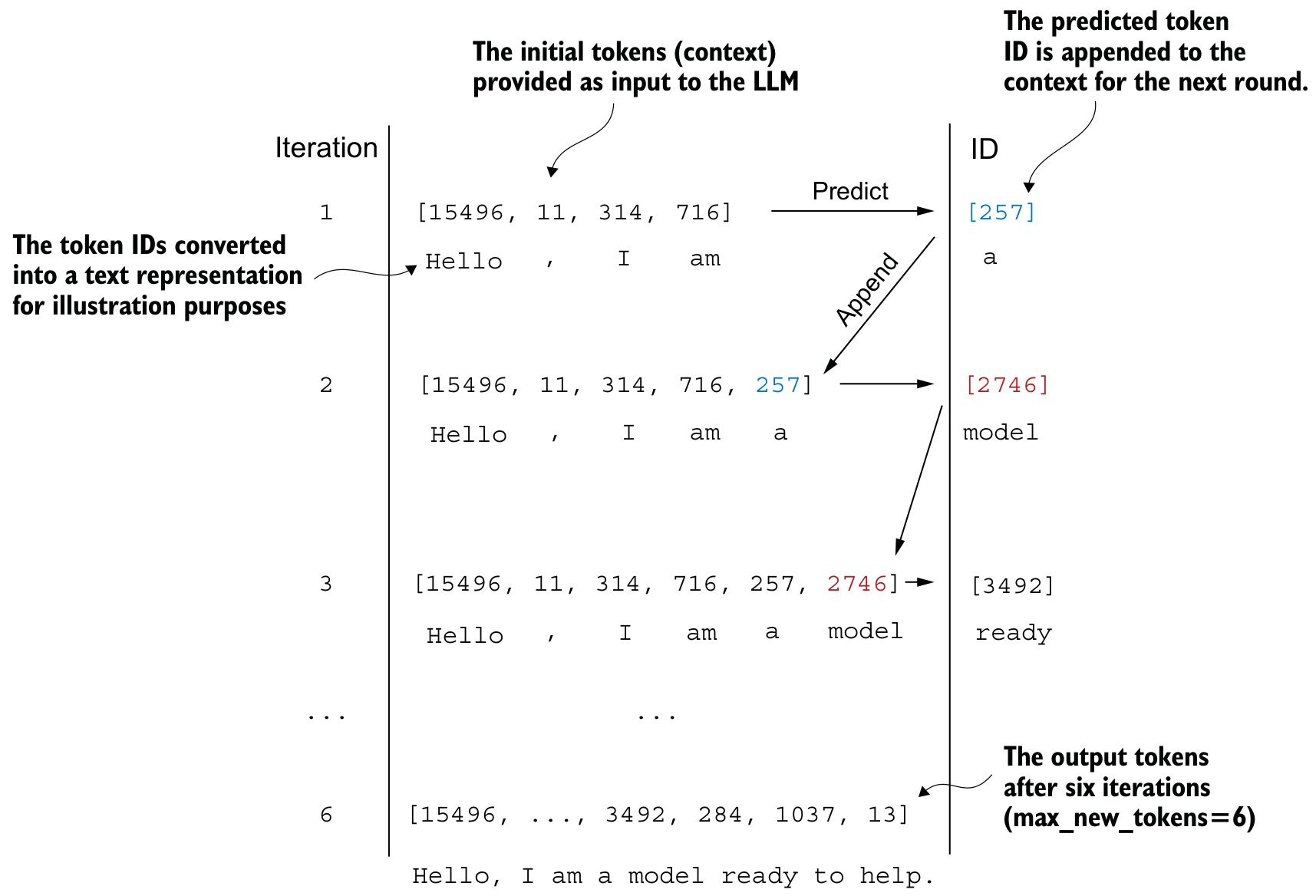
A generative model produces text one word, or token, at a time. Given the input context “Hello, I am”, the first iteration appends “a”, the second “model”, the third “ready”, and by the sixth the model has constructed the sentence “Hello, I am a model ready to help.” The input context grows with each iteration.
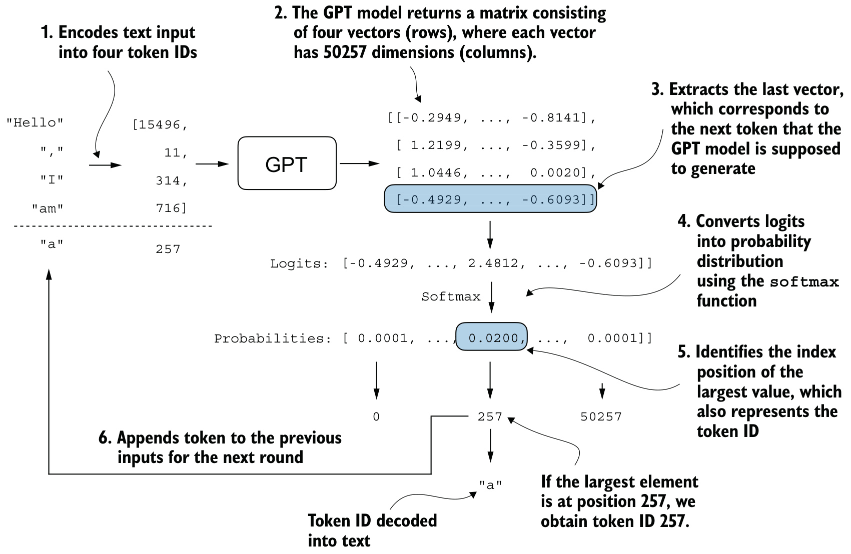
A single iteration proceeds as follows. The model outputs a matrix of vectors representing potential next tokens. The vector corresponding to the next token — the last one — is extracted and converted into a probability distribution via the softmax function. Within that vector of probability scores, the index of the highest value is located, which translates to the token ID. The token ID is decoded back into text, and appended to the previous inputs, forming a new input sequence for the subsequent iteration.
def generate_text_simple(model, idx,
                         max_new_tokens, context_size):
    for _ in range(max_new_tokens):
        idx_cond = idx[:, -context_size:]
        with torch.no_grad():
            logits = model(idx_cond)

        logits = logits[:, -1, :]
        probas = torch.softmax(logits, dim=-1)
        idx_next = torch.argmax(probas, dim=-1, keepdim=True)
        idx = torch.cat((idx, idx_next), dim=1)

    return idx
idx is a (batch, n_tokens) array of indices in the current context.
idx_cond = idx[:, -context_size:]crops the current context if it exceeds the supported context size.If the LLM supports only 5 tokens and the context size is 10, only the last 5 tokens are used as context.
logits = logits[:, -1, :]focuses only on the last time step.The shape
(batch, n_token, vocab_size)becomes(batch, vocab_size).idx_nexthas shape(batch, 1)and is concatenated to the running sequence, whose shape becomes(batch, n_tokens+1).Selecting the most probable token this way is known as greedy decoding.
torch.softmax is monotonic: it preserves the order of its inputs when transformed into outputs. The position with the highest score in the softmax output tensor is therefore the same position as in the logit tensor, and torch.argmax applied to the logits directly gives identical results. The conversion is written out because it illustrates the full process of turning logits into probabilities. It ceases to be redundant once sampling replaces the maximum.
Running it
start_context = "Hello, I am"
encoded = tokenizer.encode(start_context)
print("encoded:", encoded)
encoded_tensor = torch.tensor(encoded).unsqueeze(0)
print("encoded_tensor.shape:", encoded_tensor.shape)
The encoded IDs are [15496, 11, 314, 716], and unsqueeze(0) adds the batch dimension, giving torch.Size([1, 4]). The model is put into .eval() mode, which disables random components such as dropout that are only used during training.
model.eval()
out = generate_text_simple(
    model=model,
    idx=encoded_tensor,
    max_new_tokens=6,
    context_size=GPT_CONFIG_124M["context_length"]
)
print("Output:", out)
print("Output length:", len(out[0]))
The output token IDs are tensor([[15496, 11, 314, 716, 27018, 24086, 47843, 30961, 42348, 7267]]), of length \(10\): the four given, plus six generated. Decoding with tokenizer.decode(out.squeeze(0).tolist()) yields
Hello, I am Featureiman Byeswickattribute argueThe model generated gibberish, not the coherent Hello, I am a model ready to help. The reason is that it has not been trained. Only the GPT architecture has been implemented, and a GPT model instance initialized with random weights.
Learning outcomes
- autoregressive-greedy-generation Write the autoregressive loop that turns logits into generated text.
Concepts
- greedy-decoding
torch.argmaxover the last position’s probabilities selects one token ID per iteration, deterministically - gpt-architecture in
.eval()mode and undertorch.no_grad(), the assembled model is called repeatedly on its own output
Conclusion
GPT models are modular and built from repeating transformer blocks containing normalization, attention and feed-forward sub-layers.
Twelve blocks of identical structure, plus embeddings and an output head, account for the whole 124-million-parameter architecture, and the same
GPTModelclass produces the 345, 762 and 1,542 million parameter variants.Layer normalization and shortcut connections stabilize training and mitigate vanishing gradients.
LayerNormholds each token’s activations at mean \(0\) and variance \(1\) before each sub-layer; the two shortcut additions per block raised the first layer’s mean absolute gradient from \(0.0002\) to \(0.2217\) in the five-layer measurement.Parameter counts and memory footprints follow from the embedding dimension, the layer count and whether weight tying is used.
The raw model holds \(163{,}009{,}536\) parameters, \(621.83\) MB in float32; removing the duplicated \(50257 \times 768\) output matrix leaves \(124{,}412{,}160\).
Text generation is an iterative autoregressive loop, and requires training to produce coherent text.
Each iteration crops the context, takes the last position’s logits, applies softmax and
argmax, and appends the chosen ID. With random weights the six tokens generated from “Hello, I am” wereFeatureiman Byeswickattribute argue.
The next unit, 5 Pretraining on unlabeled data, supplies what is missing. Cross-entropy loss and perplexity measure how wrong a next-token prediction is; an AdamW training loop changes the weights in response; multinomial sampling with temperature scaling and top-\(k\) filtering replaces the deterministic argmax above; and OpenAI’s released GPT-2 tensors are mapped into this exact architecture, which is why its module names and tensor shapes were made to match.
References
- Building a Large Language Model (from scratch), Sebastian Raschka, 2024, Manning Books — Link — Page 114-149