4 Implementing a GPT model from scratch to generate text

Language Models · v1.0.0

2026-08-25 14:46:38

Where we are

From attention to a whole model

• Previous unit: attention machinery from first principles — dot-product scores, scaling by \(\sqrt{d_k}\), causal masking, dropout, and a multi-head attention module.
• That module is one sub-layer of one block.
• This unit supplies everything that surrounds attention, then runs the finished model.

Raschka opens this chapter with the same observation: “You’ve already learned and coded the multi-head attention mechanism, one of the core components of LLMs. Now, we will code the other building blocks of an LLM and assemble them into a GPT-like model that we will train in the next chapter to generate human-like text.” Assumes students remember the BPE tokenizer and embedding layers from the text-data unit.

What we will cover

• GPT architecture — a decoder-only transformer generating text one token at a time.
• Layer normalization — standardizing activations to zero mean, unit variance.
• GELU — a smooth activation, used in place of ReLU.
• Feed-forward network — expands the embedding fourfold, then projects back.
• Shortcut connections — adding a layer’s input to its output.
• Transformer block — attention and feed-forward, under pre-LayerNorm, dropout, shortcuts.
• Weight tying — sharing one matrix between token embedding and output head.
• Greedy decoding — selecting the highest-probability token at each step.

Where this sits, and what’s ahead

• Coding the model architecture is step 3 of stage 1 — after data preparation and attention, before pretraining and fine-tuning.
• We scale up to the real size: GPT-2 124M parameters, as in Radford et al., “Language Models Are Unsupervised Multitask Learners.”
• We will not train anything in this unit. Every weight stays at random initialization — the model’s output will be gibberish. That gap motivates the next unit.

A word on “parameter”: the trainable weights of the model, adjusted during training to minimize a loss function. A 2048x2048 weight matrix contributes 2048*2048 = 4,194,304 parameters — we will be counting these later.

Why GPT-2 and not GPT-3? OpenAI released the GPT-2 weights. Architecturally the two are “fundamentally the same,” GPT-3 scaled from 1.5B to 175B parameters. Lambda Labs estimates training GPT-3 would take 355 years on a single V100 GPU, or 665 years on a consumer RTX 8000.

Configuration and a dummy architecture

Top-down: fix the shape first

Fix the hyperparameters, sketch the whole model in placeholders, then fill each placeholder in.

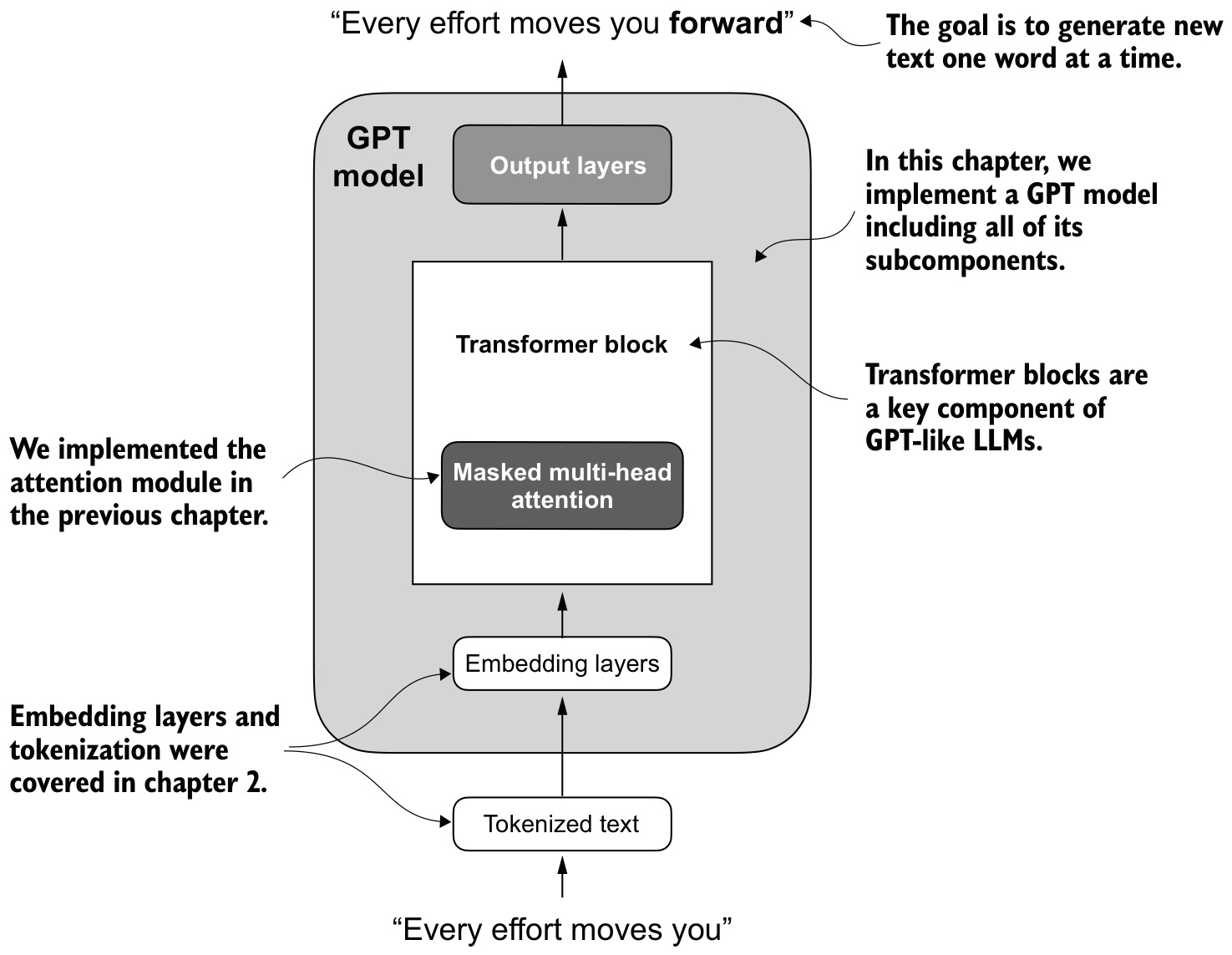
A GPT model: embedding layers plus one or more transformer blocks containing masked multi-head attention.

The configuration

The configuration collects every shape the model needs, in one place.

key	meaning	GPT-2 124M value
vocab_size	BPE vocabulary size	50,257
context_length	max tokens via positional embeddings	1,024
emb_dim	embedding dimension per token	768
n_heads	attention heads per block	12
n_layers	number of transformer blocks	12
drop_rate	dropout probability	0.1
qkv_bias	bias on Q/K/V projections	False

The skeleton

A placeholder model establishes the data path before any internals are real.

# pseudo-code
class DummyGPTModel:
    def __init__(cfg):
        tok_emb, pos_emb    = embedding tables over vocab and context length
        drop_emb            = dropout(cfg.drop_rate)
        trf_blocks           = n_layers x DummyTransformerBlock   # identity, for now
        final_norm           = DummyLayerNorm                     # identity, for now
        out_head              = linear(emb_dim -> vocab_size, no bias)

    def forward(token_ids):
        x = tok_emb(token_ids) + pos_emb(positions)
        x = drop_emb(x)
        x = trf_blocks(x)
        x = final_norm(x)
        return out_head(x)          # logits

The forward method is the whole design in six lines: embed the token IDs, add positional embeddings, apply dropout, run the blocks, normalize, project to the vocabulary. Blocks and normalization do nothing yet — they exist to be replaced later, section by section.

The shape check

Feeding two tokenized sentences (four tokens each) through the placeholder gives output shape:

\[[2,\ 4,\ 50257]\]

Two texts, four tokens each, and one logit — an unnormalized score — for every vocabulary entry at every position.

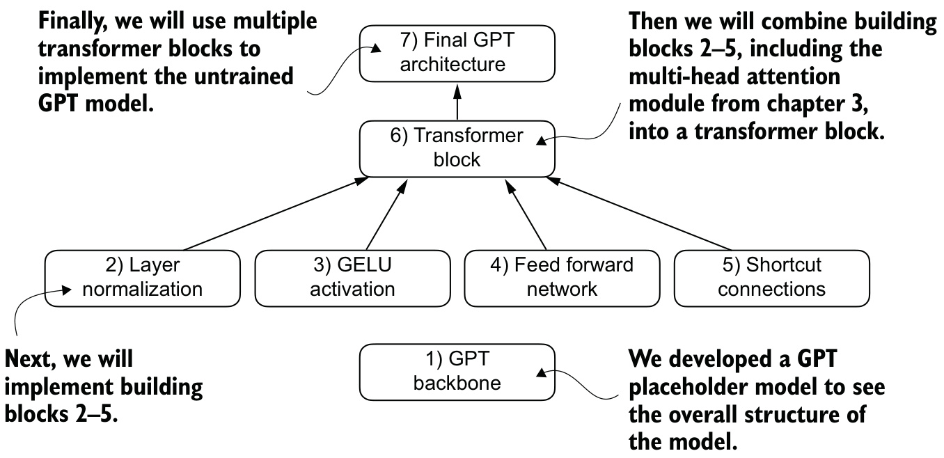
The order in which we code the GPT architecture, starting from the placeholder backbone.

Why 50,257 dimensions? Each dimension refers to a unique token in the vocabulary. Converting those vectors back into token IDs, and IDs back into words, is the last section of this unit.

Layer normalization

The problem it fixes

Deep networks are hard to train: vanishing or exploding gradients lead to unstable training dynamics and make it difficult to adjust weights effectively.

Layer normalization adjusts a layer’s activations to have mean \(0\) and unit variance.

Six activations normalized to zero mean and unit variance.

The normalization axis decides which dimension the statistic is taken over.

The operation

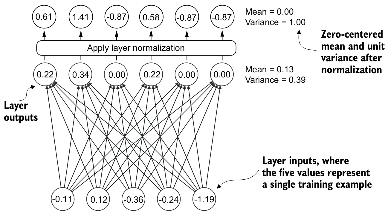
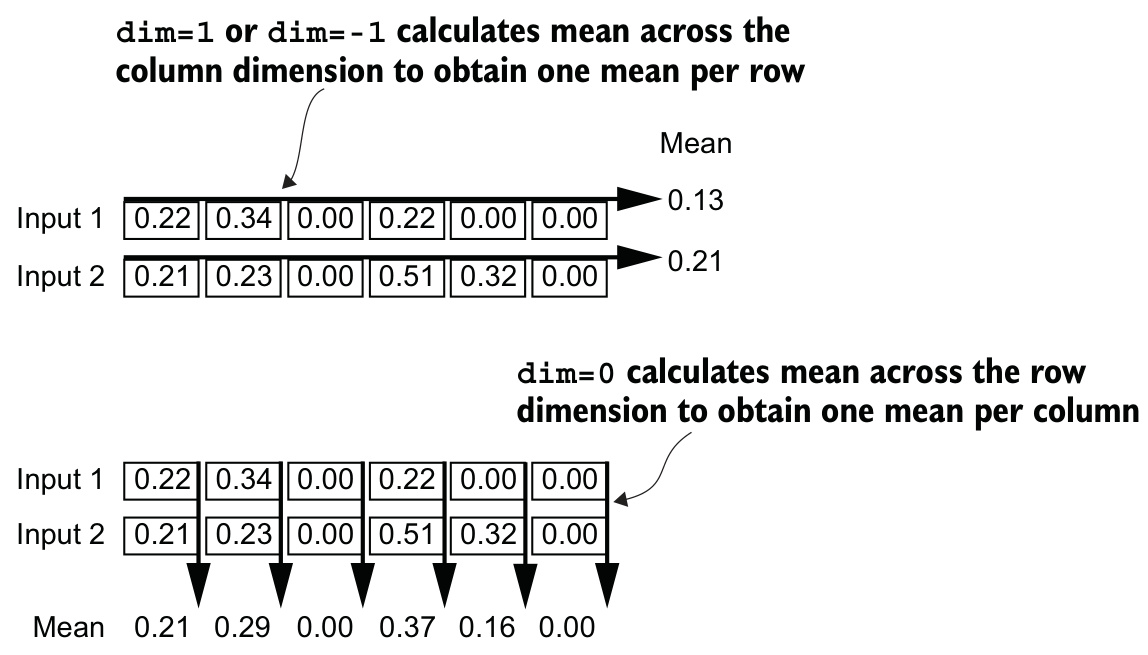
\[\hat{x} = \gamma \odot \frac{x - \mu}{\sqrt{\sigma^2 + \varepsilon}} + \beta\]

• \(\gamma\) (scale) and \(\beta\) (shift) are trainable vectors of length emb_dim.
• \(\varepsilon\) prevents division by zero.
• The statistic is taken over the feature axis — independently per token, per example — never over the batch or token axis.

For the GPT model’s three-dimensional tensors, shape [batch_size, num_tokens, embedding_size], normalization always reduces over the last (feature) axis. Batch normalization normalizes across the batch dimension instead; layer normalization’s independence from batch size gives it more flexibility and stability.

Biased variance: this divides by n rather than n-1 (no Bessel’s correction). For LLMs, where the embedding dimension is large, the difference is practically negligible — and this choice keeps compatibility with GPT-2’s own normalization layers, which used TensorFlow’s default behavior.

GELU and the feed-forward network

Two sub-layers, two jobs

Attention mixes information across token positions.

The feed-forward sub-layer does the opposite: it transforms each position on its own.

GELU

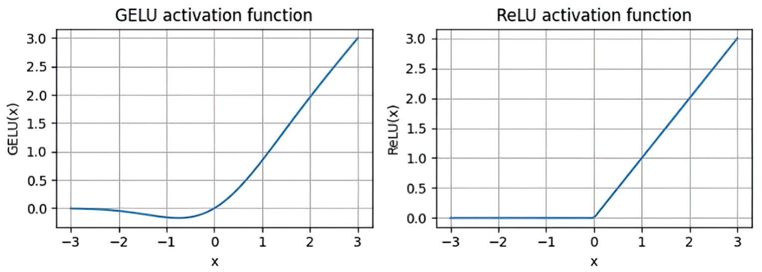
ReLU has long been the default activation, but LLMs generally use something smoother.

\[\mathrm{GELU}(x) = x \cdot \Phi(x)\]

where \(\Phi(x)\) is the standard Gaussian CDF. In practice, a cheaper curve-fit approximation is used — the same one GPT-2 was trained with:

\[\mathrm{GELU}(x) \approx 0.5 x \left(1 + \tanh\!\left[\sqrt{\tfrac{2}{\pi}}\left(x + 0.044715\,x^{3}\right)\right]\right)\]

GELU against ReLU

GELU (left) against ReLU (right).

• ReLU is piecewise linear: the input directly if positive, zero otherwise.
• GELU is smooth, with a non-zero gradient for almost all negative values.

Two consequences follow. Smoothness can lead to better optimization properties, allowing more nuanced parameter adjustments — whereas ReLU’s sharp corner at zero can make optimization harder. And because GELU gives a small, non-zero output for negative values, neurons receiving negative input can still contribute to learning, albeit to a lesser extent than positive inputs.

The feed-forward network

Two linear projections around a GELU:

# pseudo-code
def feed_forward(x, emb_dim):
    x = linear(x, emb_dim -> 4 * emb_dim)
    x = GELU(x)
    x = linear(x, 4 * emb_dim -> emb_dim)
    return x

With emb_dim = 768, the network widens each token vector to \(3072\) and narrows it back — shape is preserved end to end.

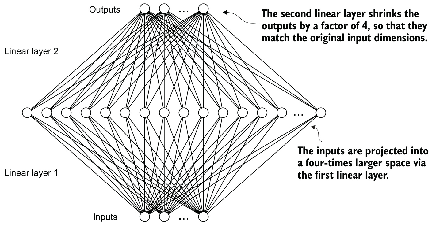
Expansion by a factor of four (768 → 3,072) and contraction back.

Why widen at all? The expansion followed by nonlinear GELU then contraction allows exploration of a richer representation space. Why insist input and output match? Uniform dimensions simplify the architecture, enabling stacking of multiple layers without adjusting dimensions between them. The module applies identically and independently at every token position; it accommodates variable batch sizes and token counts, but the embedding size is fixed at initialization.

Shortcut connections and gradient flow

The vanishing gradient problem

Shortcut connections (skip / residual connections) were originally proposed for deep computer-vision networks to mitigate vanishing gradients.

The vanishing gradient problem: gradients become progressively smaller as they propagate backward through layers, making it difficult to train earlier layers.

The mechanism

A shortcut creates an alternative, shorter path for the gradient: it skips one or more layers by adding the output of one layer to the output of a later layer.

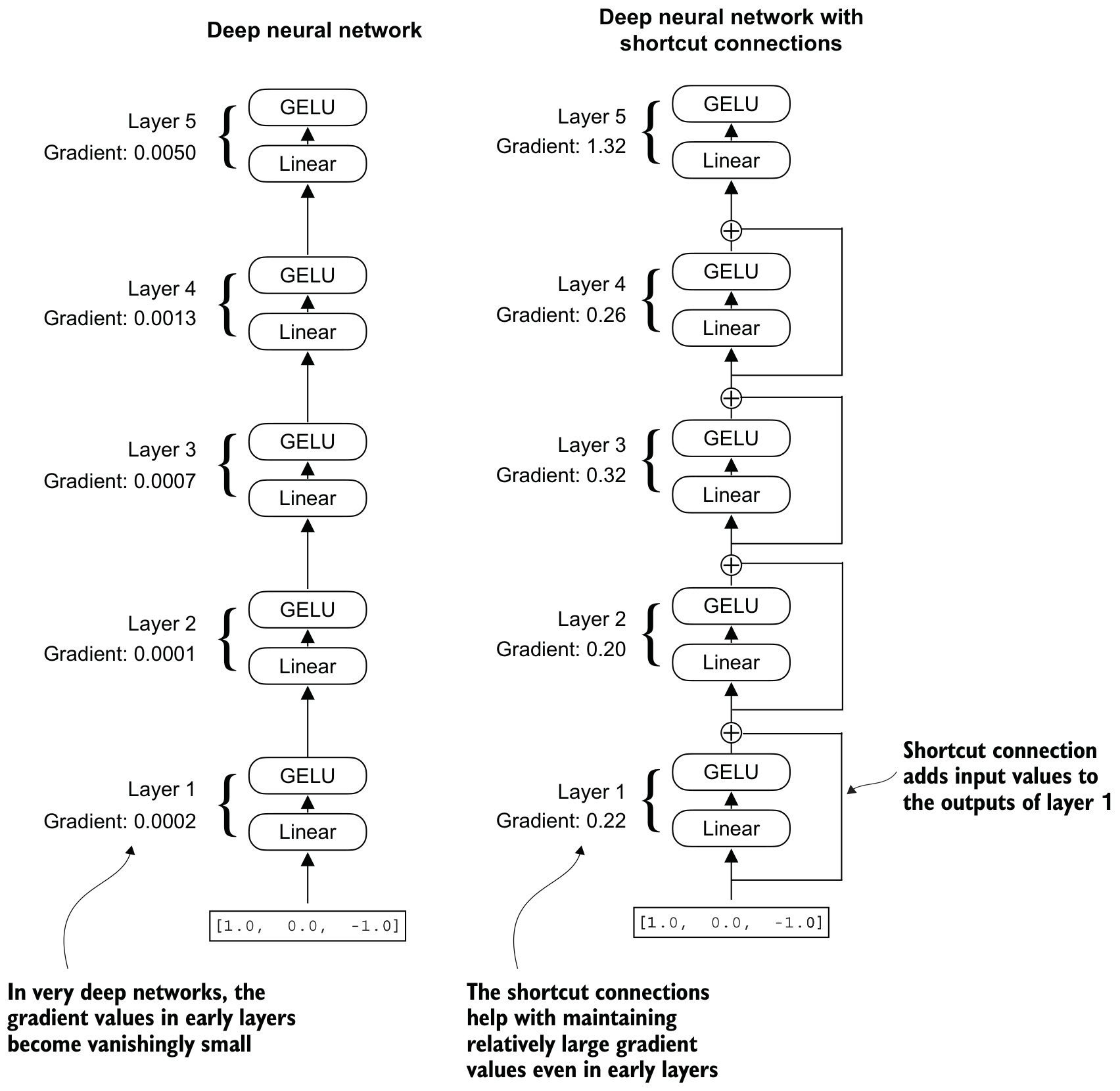
Five layers without shortcuts (left) and with them (right), annotated with mean absolute gradient at each layer.

The argument is empirical: measure the problem, then measure the fix, on a five-layer test network. Without shortcuts, the mean absolute gradient shrinks by roughly an order of magnitude from the last layer to the first. With shortcuts, the gradient at the first layer rises by roughly a factor of a thousand and stabilizes as we progress toward the first layer, rather than vanishing.

Why this matters for our GPT

Our model stacks twelve transformer blocks, each with two sub-layers.

Shortcut connections are a core building block of very large models such as LLMs — they help ensure consistent gradient flow across layers. Every sub-layer in the next section is wrapped in one.

The transformer block

The repeating unit

The transformer block is repeated a dozen times in GPT-2 124M. It combines multi-head attention, layer normalization, dropout, feed-forward layers, and GELU.

• The self-attention mechanism identifies relationships between elements in the sequence.
• The feed-forward network modifies the data individually at each position.

The module

# pseudo-code
def transformer_block(x):
    shortcut = x
    x = layer_norm(x)
    x = multi_head_attention(x)
    x = dropout(x)
    x = x + shortcut

    shortcut = x
    x = layer_norm(x)
    x = feed_forward(x)
    x = dropout(x)
    x = x + shortcut
    return x

One pattern, applied twice

1. Save a shortcut copy of the input.
2. Normalize.
3. Apply the operation, then dropout.
4. Add the shortcut back.

The operation is masked multi-head attention the first time, the feed-forward network the second. Only the layer-norm parameters differ between the two.

Pre-LayerNorm

Normalization comes before each operation, not after — this is Pre-LayerNorm.

Older architectures, including the original transformer, applied normalization after attention and feed-forward — Post-LayerNorm — which often leads to worse training dynamics.

Shape in, shape out

The block preserves shape: [batch, tokens, emb_dim] in, [batch, tokens, emb_dim] out.

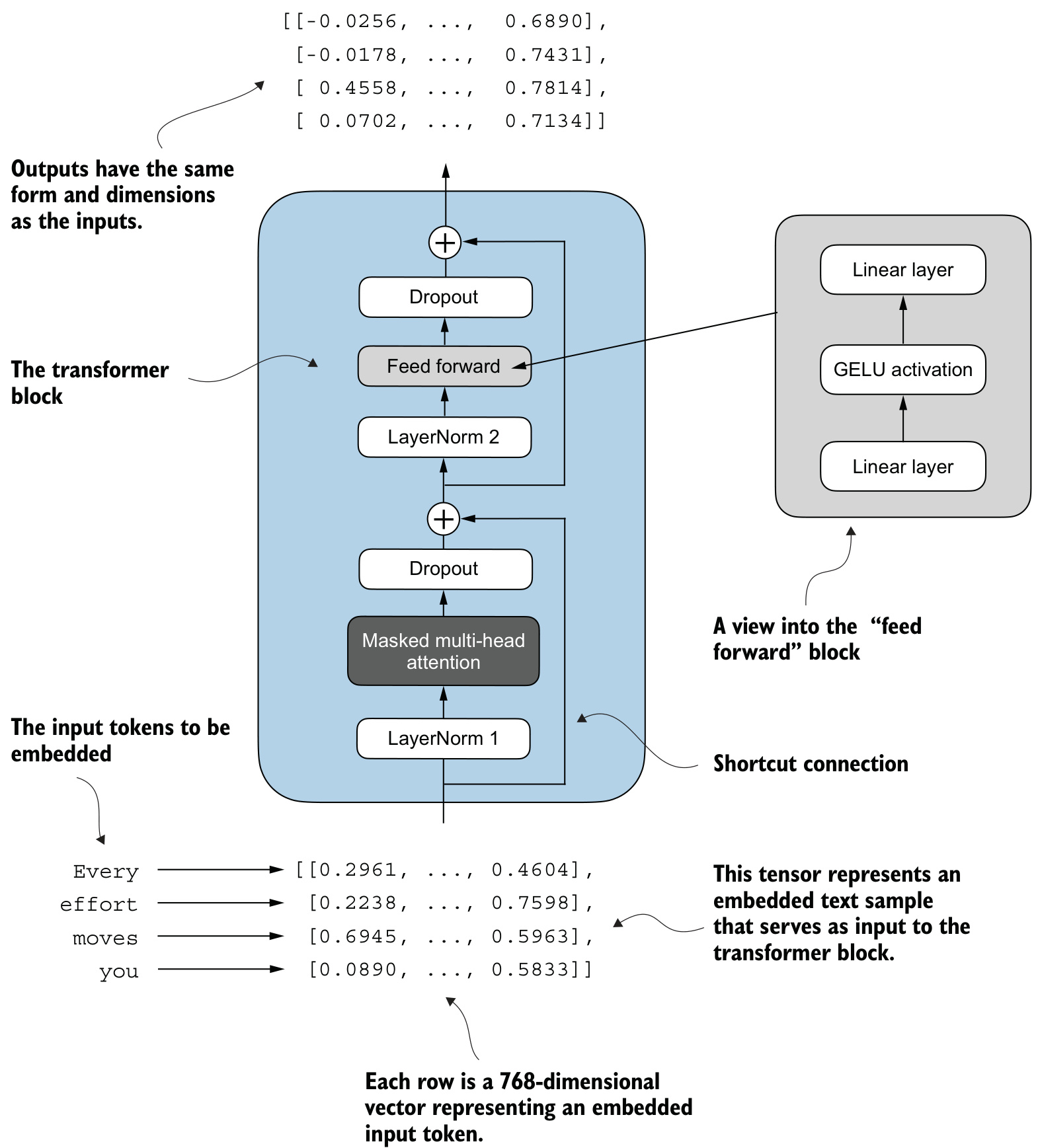
Each row is one token’s 768-dimensional vector; output vectors keep the same dimension as the input.

Shape preservation is not incidental — it is what lets blocks stack without any dimension bookkeeping. What changes is the content: while the physical dimensions stay unchanged, each output vector is re-encoded to integrate contextual information from across the entire input sequence.

Key ideas

• Two residual sub-layers, one pattern: norm, operate, drop, add.
• Attention mixes across positions; the feed-forward network transforms each position alone.
• Pre-LayerNorm, not Post-LayerNorm — the ordering GPT-2 uses.
• The block is shape-preserving, which is what makes stacking twelve of them trivial.

Assembling the GPT model

Replacing the placeholders

Everything is now built. The full GPT model is the placeholder skeleton with its two placeholders replaced by real transformer blocks and real layer normalization.

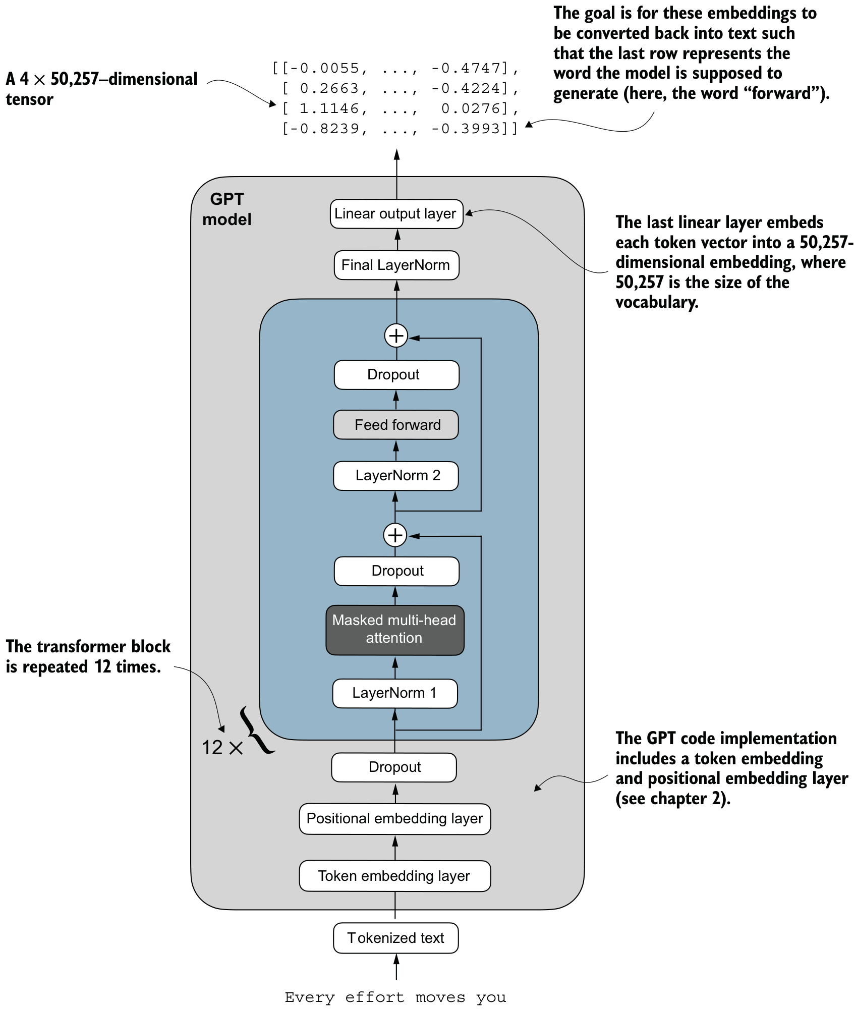
The complete GPT model: token + positional embeddings, twelve transformer blocks, a final layer norm, and a linear output head.

The module

# pseudo-code
class GPTModel:
    def __init__(cfg):
        tok_emb, pos_emb = embedding tables over vocab and context length
        drop_emb          = dropout(cfg.drop_rate)
        trf_blocks         = n_layers x TransformerBlock(cfg)
        final_norm          = LayerNorm(cfg.emb_dim)
        out_head             = linear(emb_dim -> vocab_size, no bias)

    def forward(token_ids):
        x = tok_emb(token_ids) + pos_emb(positions)
        x = drop_emb(x)
        x = trf_blocks(x)
        x = final_norm(x)
        return out_head(x)     # logits

Thanks to TransformerBlock, GPTModel is relatively small and compact.

Input, body, head

• Input. Embedding layers convert token indices into dense vectors and add positional information — the positional embeddings are learnable, not a fixed sinusoid. Embedding dropout follows.
• Body. A sequential stack of transformer blocks: twelve for GPT-2 small, forty-eight for the largest GPT-2 (1,542M parameters).
• Head. A final layer normalization, then a linear output head without bias, projecting into the vocabulary space.

Feeding the same two-sentence batch through the assembled model still gives output shape [2, 4, 50257].

Logits are not probabilities: the forward pass computes unnormalized scores for the next token. Turning them into tokens is the last section of this unit; turning them into a training signal belongs to the next.

Counting parameters and memory

More parameters than expected

Summing every parameter tensor in the assembled model gives \(163{,}009{,}536\) — not the 124 million we set out to build.

Where do the extra 39 million come from?

Weight tying

Weight tying was used in the original GPT-2: it reuses the weights from the token embedding layer in the output layer.

• Token embedding matrix and output-head matrix: same shape, [vocab_size, emb_dim], about \(38.6\) million entries each.
• Removing the duplicate copy brings the count to \(124{,}412{,}160\) — matching GPT-2’s published size.

We do not tie the weights

Weight tying reduces memory footprint and computational complexity, but separate token embedding and output layers give better training and model performance in practice — the same is true for modern LLMs. Our model genuinely holds 163 million parameters; 124M describes OpenAI’s tied version.

Memory

At 32-bit floats, 4 bytes per parameter:

\[163{,}009{,}536 \text{ params} \;\approx\; 621.83\text{ MB}\]

That figure covers the weights alone, before optimizer state or activations.

Scaling the configuration

The same architecture produces every GPT-2 size — only the configuration changes.

Model	emb_dim	n_layers	n_heads
GPT-2 small	768	12	12
GPT-2 medium	1,024	24	16
GPT-2 large	1,280	36	20
GPT-2 XL	1,600	48	25

Exercise 4.1 asks you to compare the parameter counts of the feed-forward module and the multi-head attention module within one block. Exercise 4.2 asks you to instantiate the three larger variants without any code modifications besides updating the configuration file.

Generating text autoregressively

From one distribution to a generator

A model that emits one distribution becomes a text generator by being called repeatedly on its own output.

Given “Hello, I am”, the model predicts a token, appends it, and predicts again — by the sixth iteration, it has constructed a complete sentence.

One generation step: encode, run the model, take the last position’s logits, softmax, pick the token ID, append.

The loop

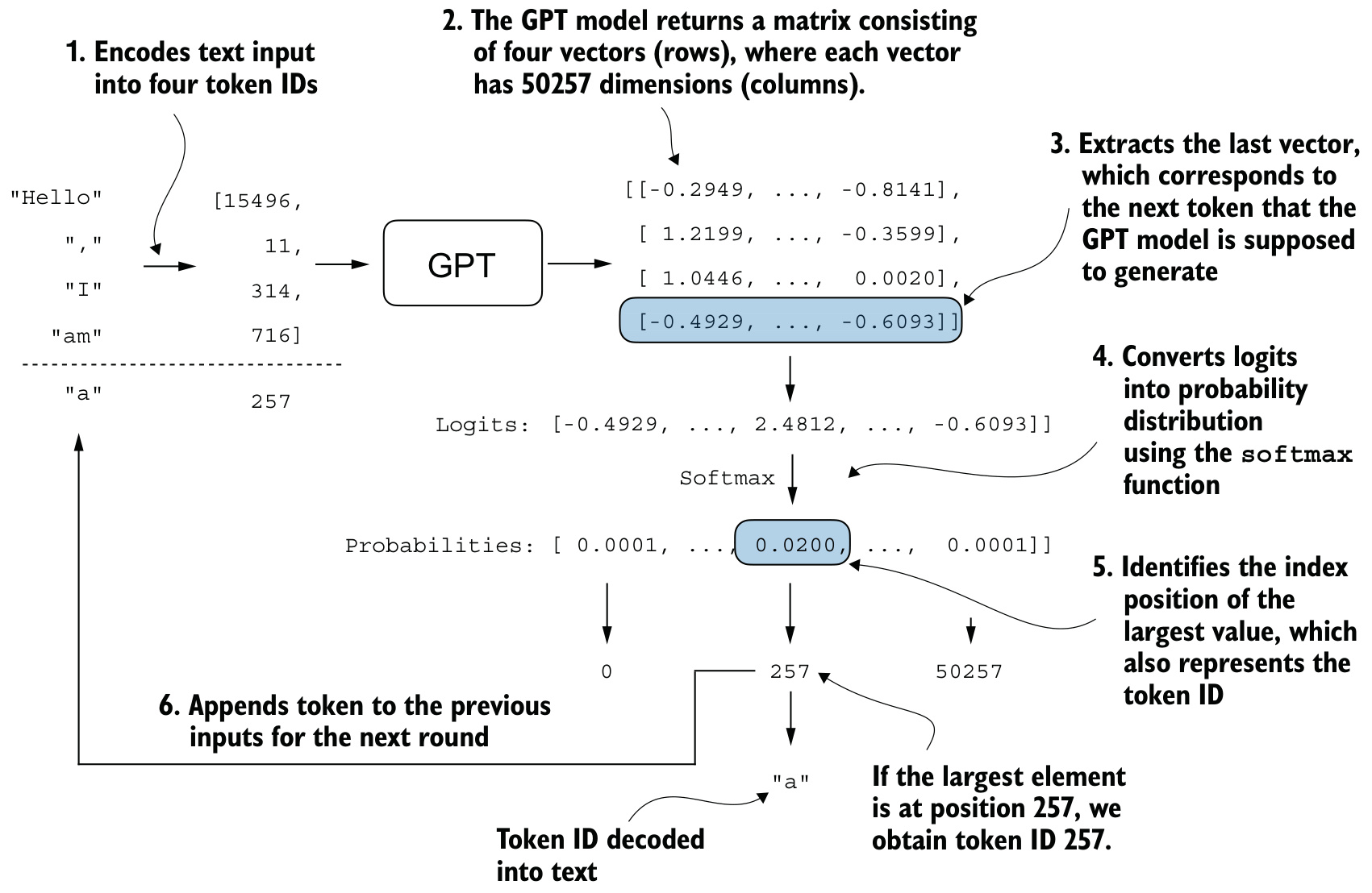
# pseudo-code
def generate(model, idx, max_new_tokens, context_size):
    for _ in range(max_new_tokens):
        idx_cond = idx[-context_size:]        # crop to the model's context window
        logits    = model(idx_cond)
        logits     = logits[last position]     # only the next-token prediction matters
        probs       = softmax(logits)
        next_id      = argmax(probs)             # greedy decoding
        idx           = concat(idx, next_id)
    return idx

Five things happen per iteration

• The running context is cropped to the model’s supported window.
• The forward pass runs without tracking gradients — none are needed at inference time.
• Only the last position’s logits are kept — the prediction for the next token.
• Softmax then argmax selects the single most probable token ID: greedy decoding.
• The new token is appended, and the loop repeats.

The softmax step is technically redundant here: softmax is monotonic, so the position with the highest score in the softmax output is the same position in the logit tensor. It’s written out to make the logits-to-probabilities path explicit — it stops being redundant in the next unit, where sampling replaces the maximum.

Running it

Encoding “Hello, I am” and running six generation steps through the untrained model produces:

Hello, I am Featureiman Byeswickattribute argue

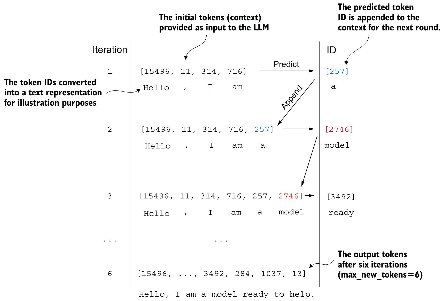
Six iterations of the token prediction cycle, each appending its prediction to the input.

Gibberish, and expectedly so: we have only implemented the architecture and initialized random weights. Architecture alone does not produce language.

What you can now build

The architecture, end to end

• Specify a GPT configuration and describe the architecture top-down, from placeholders to working components.
• Explain layer normalization, GELU, the feed-forward network, and residual shortcuts, and what each contributes to stable optimization.
• Compose them with masked multi-head attention into a transformer block, stack twelve into a GPT model, and reason about its parameter count and memory footprint.
• Describe how the model generates text with greedy decoding.

What is missing: nothing in this unit measures how wrong an output is, and nothing changes a weight in response.

Key ideas

• GPT models are modular: embeddings, a stack of identical transformer blocks, a final norm, a linear head.
• Layer normalization stabilizes training by keeping each layer’s outputs at a consistent mean and variance.
• Shortcut connections mitigate vanishing gradients — measured directly, the first layer’s mean gradient rises from \(0.00020\) to \(0.2217\) once shortcuts are added.
• Transformer blocks combine masked multi-head attention with a GELU feed-forward network; both sub-layers preserve \([B, T, \text{emb\_dim}]\).
• Parameter counts depend on weight tying: \(163{,}009{,}536\) untied vs. \(124{,}412{,}160\) tied.
• Without training, a correct architecture with random weights produces incoherent text.

Where next

Next: 5 Pretraining on unlabeled data.

It defines cross-entropy loss and perplexity, builds a training loop around AdamW, and shows the overfitting a small corpus produces. It replaces greedy decoding with temperature scaling and top-\(k\) sampling, adds checkpointing, and loads OpenAI’s pretrained GPT-2 weights into the architecture we just wrote.

That last step is why the details of this unit mattered: the module names and tensor shapes match GPT-2, so trained weights load straight into our code. For the concrete PyTorch implementation behind each component, see chapter 4 of Building a Large Language Model (from scratch).