Lecture notes — 5 Pretraining on unlabeled data
ver. 1.2.0, 5_pretraining_on_unlabeled_data
← 5 Pretraining on unlabeled data
ver. 1.2.0 · 2026-09-02 16:27:35
From a random model to a trained one
The previous unit, 4 Implementing a GPT model from scratch to generate text, ended with a complete GPTModel and a greedy generation loop. Its output was noise, because every weight was a random initialization. Nothing was missing from the architecture; what was missing was a numerical measure of error, an optimization procedure that reduces it, a decoding rule less rigid than argmax, and a way to keep the result.
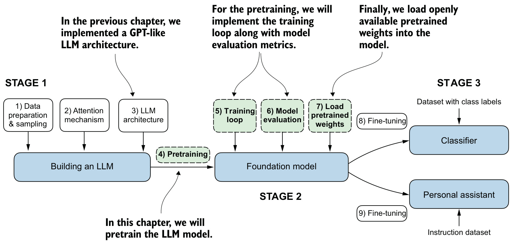
Chapter 5 of Building a Large Language Model (from scratch) supplies those four pieces. It is stage 2 of building an LLM: pretraining the architecture on unlabeled text, then loading openly available pretrained weights into it.
Weights in this chapter means the trainable parameters a layer stores. After new_layer = torch.nn.Linear(...), they are reachable as new_layer.weight; model.parameters() returns weights and biases together, which is what the optimizer is handed.
The corpus is a single public-domain short story, so every experiment finishes in minutes on a laptop. That choice makes overfitting visible rather than hypothetical, and it is the reason the chapter ends by importing OpenAI’s weights instead of earning comparable ones.
Learning outcomes
- cross-entropy-loss-and-perplexity Compute the text generation loss from logits and interpret it as perplexity.
- pretraining-loop-with-adamw Write a complete pretraining loop that optimizes an LLM with AdamW.
- loading-openai-gpt2-weights Map OpenAI’s released GPT-2 weights into your own PyTorch implementation.
Learning outcomes
cross-entropy-loss-and-perplexity— Compute the text generation loss from logits and interpret it as perplexity.train-and-validation-loss-evaluation— Split a corpus into training and validation loaders and measure the loss over each.pretraining-loop-with-adamw— Write a complete pretraining loop that optimizes an LLM with AdamW.diagnosing-overfitting— Read training and validation loss curves to recognize memorization.temperature-scaling— Replace greedy decoding with multinomial sampling controlled by a temperature.top-k-sampling-and-the-generate-function— Restrict sampling to the top-k candidates and combine the decoding controls into one generate function.checkpointing-model-and-optimizer— Save and restore model weights together with optimizer state.loading-openai-gpt2-weights— Map OpenAI’s released GPT-2 weights into your own PyTorch implementation.
Concepts introduced
- Cross entropy loss — the negative average log probability the model assigns to the target tokens.
- Perplexity — the exponential of the loss, read as the effective vocabulary size the model is undecided among.
- AdamW optimizer — a variant of Adam whose weight decay penalizes large weights independently of the gradient update.
- Greedy decoding — selecting the highest-probability token at every step with
torch.argmax. - Temperature scaling — dividing the logits by a constant \(T > 0\) before
softmax, which sharpens or flattens the distribution. - Top-k sampling — keeping the \(k\) largest logits and masking the rest with \(-\infty\), so excluded tokens receive probability zero.
- Checkpoint saving and loading — serializing a
state_dictfor the model and for the optimizer, so a session can be resumed. - Weight tying — reusing the token embedding matrix as the output projection, so one tensor serves two positions in the network.
From logits to a loss
The model is instantiated from the configuration of the previous unit with one change:
GPT_CONFIG_124M = {
    "vocab_size": 50257,
    "context_length": 256,
    "emb_dim": 768,
    "n_heads": 12,
    "n_layers": 12,
    "drop_rate": 0.1,
    "qkv_bias": False
}
torch.manual_seed(123)
model = GPTModel(GPT_CONFIG_124M)
model.eval()
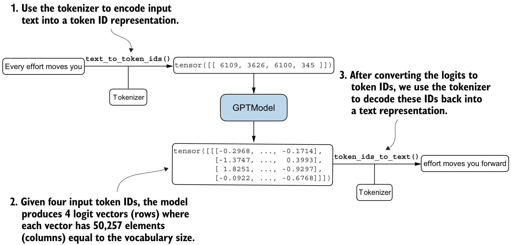
The context length is shortened from 1,024 to 256 tokens, which reduces the computational demand enough to train on a standard laptop. Two helpers convert between text and token IDs, from listing 5.1:
def text_to_token_ids(text, tokenizer):
    encoded = tokenizer.encode(text, allowed_special={'<|endoftext|>'})
    encoded_tensor = torch.tensor(encoded).unsqueeze(0)
    return encoded_tensor

def token_ids_to_text(token_ids, tokenizer):
    flat = token_ids.squeeze(0)
    return tokenizer.decode(flat.tolist())
.unsqueeze(0) adds the batch dimension; .squeeze(0) removes it. Run through generate_text_simple, the untrained model emits Every effort moves you rentingetic wasn? refres RexMeChicular stren.
The manual derivation
Two examples are used, already mapped to token IDs, with targets that are the inputs shifted one position forward:
inputs = torch.tensor([[16833, 3626, 6100],   # ["every effort moves",
                       [40,    1107, 588]])   #  "I really like"]

targets = torch.tensor([[3626, 6100, 345  ],  # [" effort moves you",
                        [1107,  588, 11311]]) #  " really like chocolate"]
The forward pass and softmax give probas of shape torch.Size([2, 3, 50257]). The probability the model assigned to each target token is indexed out directly:
text_idx = 0
target_probas_1 = probas[text_idx, [0, 1, 2], targets[text_idx]]
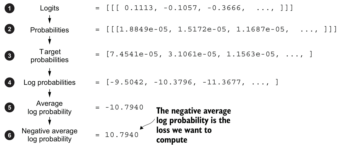
For the two batches these are tensor([7.4541e-05, 3.1061e-05, 1.1563e-05]) and tensor([1.0337e-05, 5.6776e-05, 4.7559e-06]) — close to \(1/50257 \approx 0.00002\), which is where an untrained model’s probabilities sit. Applying torch.log, averaging, and multiplying by \(-1\):
log_probas = torch.log(torch.cat((target_probas_1, target_probas_2)))
avg_log_probas = torch.mean(log_probas)
neg_avg_log_probas = avg_log_probas * -1
The average log probability is tensor(-10.7940), so the loss is tensor(10.7940). Cross entropy loss measures the difference between two probability distributions — the true token distribution and the model’s predicted one — and in this discrete setting it equals that negative average log probability. Training drives it toward 0. The logarithm is taken because working with logarithms of probability scores is more manageable in mathematical optimization than handling the scores directly.
The library version
torch.nn.functional.cross_entropy performs all six steps, but it expects the batch dimension folded in:
logits_flat = logits.flatten(0, 1)
targets_flat = targets.flatten()
loss = torch.nn.functional.cross_entropy(logits_flat, targets_flat)
logits of shape torch.Size([2, 3, 50257]) becomes torch.Size([6, 50257]), and targets of torch.Size([2, 3]) becomes torch.Size([6]). The result is tensor(10.7940) — the same number as the manual computation.
Perplexity is the exponential of the loss, perplexity = torch.exp(loss), here tensor(48725.8203). It signifies the effective vocabulary size about which the model is uncertain at each step: this model is as undecided as if it were choosing among 48,725 of its 50,257 tokens.
Key ideas
- The loss is computed from the probability assigned to the target token, not from the token the model would have chosen.
cross_entropyrequires the logits flattened over the batch dimension and the targets flattened to one dimension.- Loss and perplexity are the same measurement; \(\text{perplexity} = e^{\text{loss}}\) puts it on the scale of a vocabulary count.
Learning outcomes
- cross-entropy-loss-and-perplexity Compute the text generation loss from logits and interpret it as perplexity.
Concepts
- cross-entropy-loss the negative average log probability of the target tokens, obtained from softmax, indexing, logarithm, mean and negation, and reproduced by
torch.nn.functional.cross_entropy - perplexity \(e^{\text{loss}}\), the effective number of vocabulary tokens the model is undecided among at each step
- greedy-decoding
generate_text_simpleselects the highest-probability token withargmax, which is what produces the untrained model’s output here
Training and validation losses
The corpus is “The Verdict”, a short story by Edith Wharton in the public domain, which sidesteps usage rights and is small enough to run in minutes without a high-end GPU:
total_characters = len(text_data)
total_tokens = len(tokenizer.encode(text_data))
This prints Characters: 20479 and Tokens: 5145. The split reserves 90% for training:
train_ratio = 0.90
split_idx = int(train_ratio * len(text_data))
train_data = text_data[:split_idx]
val_data = text_data[split_idx:]
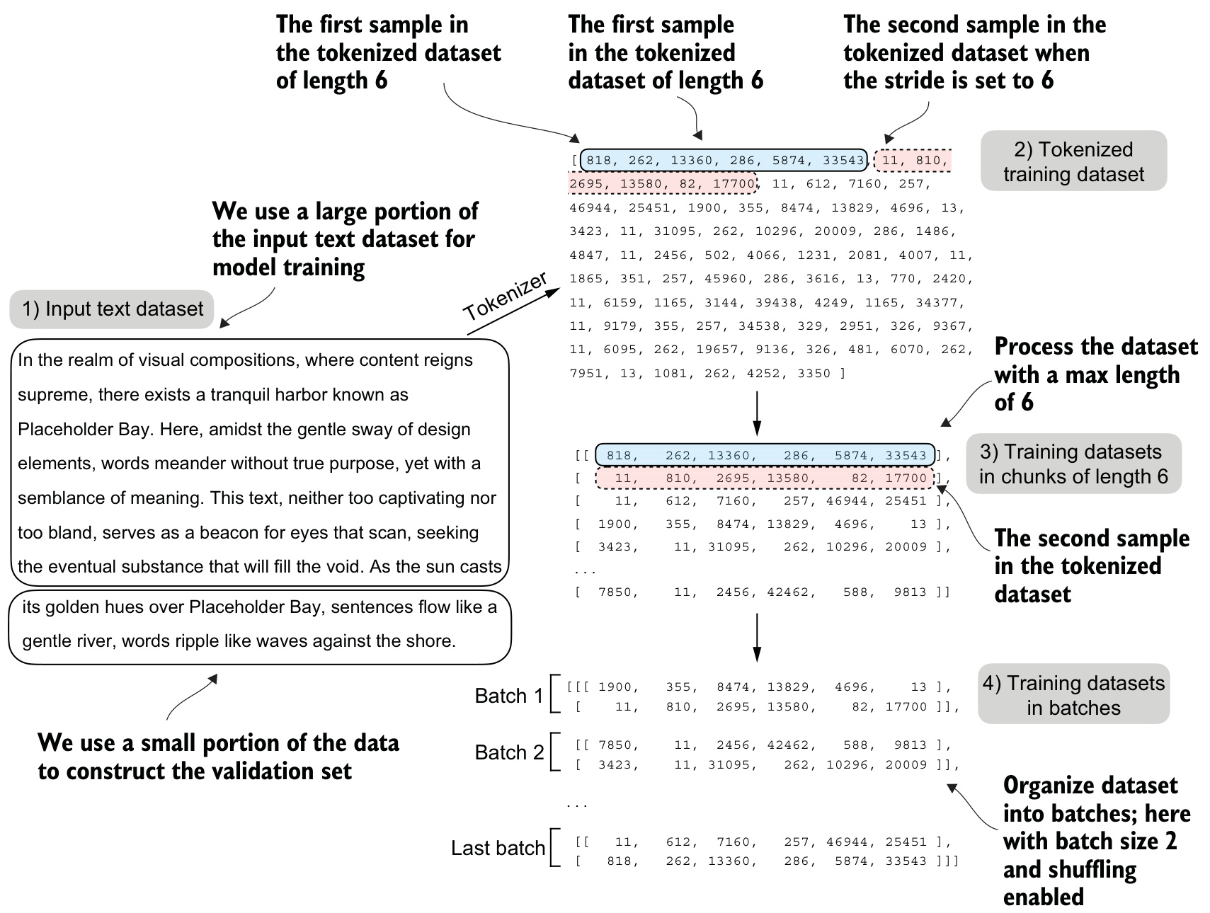
Each part is handed to create_dataloader_v1 from the data-preparation unit, with max_length and stride both set to the 256-token context length so that the LLM sees texts as long as it supports:
train_loader = create_dataloader_v1(
    train_data,
    batch_size=2,
    max_length=GPT_CONFIG_124M["context_length"],
    stride=GPT_CONFIG_124M["context_length"],
    drop_last=True,
    shuffle=True,
    num_workers=0
)
The validation loader differs in drop_last=False and shuffle=False. Iterating them yields nine training batches of torch.Size([2, 256]) and a single validation batch of the same shape. The batch size of 2 is a concession to the small dataset; in practice batch sizes of 1,024 or larger are not uncommon.
One batch, then a whole loader
Device handling is isolated in a single function:
def calc_loss_batch(input_batch, target_batch, model, device):
    input_batch = input_batch.to(device)
    target_batch = target_batch.to(device)
    logits = model(input_batch)
    loss = torch.nn.functional.cross_entropy(
        logits.flatten(0, 1), target_batch.flatten()
    )
    return loss
Listing 5.2 averages that over a loader:
def calc_loss_loader(data_loader, model, device, num_batches=None):
    total_loss = 0.
    if len(data_loader) == 0:
        return float("nan")
    elif num_batches is None:
        num_batches = len(data_loader)
    else:
        num_batches = min(num_batches, len(data_loader))
    for i, (input_batch, target_batch) in enumerate(data_loader):
        if i < num_batches:
            loss = calc_loss_batch(
                input_batch, target_batch, model, device
            )
            total_loss += loss.item()
        else:
            break
    return total_loss / num_batches
The min(num_batches, len(data_loader)) line is the guard against being asked for more batches than the loader holds; num_batches exists so that an evaluation during training can be made cheaper than a full pass.
Applied to the untrained model under torch.no_grad(), with device = torch.device("cuda" if torch.cuda.is_available() else "cpu"), the result is a training loss of 10.98755347829183 and a validation loss of 10.98110580444336. Both are near the value expected of a model with no preference among tokens.
The 7 billion parameter Llama 2 model required 184,320 GPU hours on A100 GPUs, processing 2 trillion tokens. At the time of writing, an 8 × A100 cloud server on AWS costs around $30 per hour, which puts the total training cost at around $690,000 — 184,320 hours divided by 8, then multiplied by $30.
Learning outcomes
- train-and-validation-loss-evaluation Split a corpus into training and validation loaders and measure the loss over each.
Concepts
- cross-entropy-loss
calc_loss_batchcomputes it for one batch on a chosen device, andcalc_loss_loaderaverages it across a whole loader
The pretraining loop
The loop is the standard PyTorch procedure: iterate epochs, iterate batches, reset the gradients, compute the loss, backpropagate, update the weights. Listing 5.3 adds the two monitoring steps that make progress readable:
def train_model_simple(model, train_loader, val_loader,
                       optimizer, device, num_epochs,
                       eval_freq, eval_iter, start_context, tokenizer):
    train_losses, val_losses, track_tokens_seen = [], [], []
    tokens_seen, global_step = 0, -1

    for epoch in range(num_epochs):
        model.train()
        for input_batch, target_batch in train_loader:
            optimizer.zero_grad()
            loss = calc_loss_batch(
                input_batch, target_batch, model, device
            )
            loss.backward()
            optimizer.step()
            tokens_seen += input_batch.numel()
            global_step += 1

            if global_step % eval_freq == 0:
                train_loss, val_loss = evaluate_model(
                    model, train_loader, val_loader, device, eval_iter)
                train_losses.append(train_loss)
                val_losses.append(val_loss)
                track_tokens_seen.append(tokens_seen)
                print(f"Ep {epoch+1} (Step {global_step:06d}): "
                      f"Train loss {train_loss:.3f}, "
                      f"Val loss {val_loss:.3f}"
                )

        generate_and_print_sample(
            model, tokenizer, device, start_context
        )
    return train_losses, val_losses, track_tokens_seen
optimizer.zero_grad() comes first because gradients accumulate across backward() calls; omitting it adds the previous batch’s gradients to the current update. Evaluation is delegated to a function that switches the model out of training mode:
def evaluate_model(model, train_loader, val_loader, device, eval_iter):
    model.eval()
    with torch.no_grad():
        train_loss = calc_loss_loader(
            train_loader, model, device, num_batches=eval_iter
        )
        val_loss = calc_loss_loader(
            val_loader, model, device, num_batches=eval_iter
        )
    model.train()
    return train_loss, val_loss
model.eval() disables dropout, so the measurement is stable and reproducible; torch.no_grad() disables gradient tracking, which is not required during evaluation and reduces the computational overhead. Both are undone before returning. generate_and_print_sample is the companion for qualitative inspection: it reads context_size = model.pos_emb.weight.shape[0], calls generate_text_simple with max_new_tokens=50, and prints the decoded text with decoded_text.replace("\n", " ").
Adam optimizers are a popular choice for training deep neural networks. AdamW is a variant of Adam that improves the weight decay approach, which aims to minimize model complexity and prevent overfitting by penalizing larger weights. AdamW is therefore frequently used in the training of LLMs.
The run itself:
torch.manual_seed(123)
model = GPTModel(GPT_CONFIG_124M)
model.to(device)
optimizer = torch.optim.AdamW(
      model.parameters(),
      lr=0.0004, weight_decay=0.1
)
num_epochs = 10
train_losses, val_losses, tokens_seen = train_model_simple(
    model, train_loader, val_loader, optimizer, device,
    num_epochs=num_epochs, eval_freq=5, eval_iter=5,
    start_context="Every effort moves you", tokenizer=tokenizer
)
Ten epochs take about 5 minutes on a MacBook Air or a similar laptop. The training loss starts at 9.781 and converges to 0.391. The validation loss starts at 9.933 and remains at 6.452 after the tenth epoch.
Reading the curves
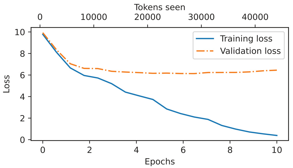
Both losses improve during the first epoch, then diverge past the second. The training loss continuing to fall while the validation loss stagnates is overfitting to the training set. The memorization is verifiable rather than inferred: the generated snippet quite insensible to the irony can be found in the “The Verdict” text file. With 5,145 tokens and ten passes over them, the model reproduces the story instead of generalizing. Common practice is to train on a much larger dataset for only one epoch.
Learning outcomes
- pretraining-loop-with-adamw Write a complete pretraining loop that optimizes an LLM with AdamW.
- diagnosing-overfitting Read training and validation loss curves to recognize memorization.
- train-and-validation-loss-evaluation Split a corpus into training and validation loaders and measure the loss over each.
Concepts
- adamw-optimizer
torch.optim.AdamW(model.parameters(), lr=0.0004, weight_decay=0.1)supplies the weight update, its decoupled weight decay penalizing large weights - cross-entropy-loss the per-batch loss supplies the gradients, and its training and validation values across epochs are what reveal memorization
Temperature scaling
Inference with a model of this size does not require a GPU, so the trained model is moved back and put in evaluation mode to turn off dropout:
model.to("cpu")
model.eval()
Twenty-five tokens from generate_text_simple on the start context "Every effort moves you" give
Every effort moves you know," was one of the axioms he laid down across the
Sevres and silver of an exquisitely appointed lun
Greedy decoding — selecting the largest probability score among all tokens in the vocabulary with torch.argmax — is deterministic. Running the same call again on the same start context produces the same passage, which for this model is a memorized one.
Probabilistic sampling
A nine-token vocabulary makes the alternative concrete:
vocab = {
    "closer": 0,
    "every": 1,
    "effort": 2,
    "forward": 3,
    "inches": 4,
    "moves": 5,
    "pizza": 6,
    "toward": 7,
    "you": 8,
}
inverse_vocab = {v: k for k, v in vocab.items()}
Given the start context "every effort moves you", the next-token logits are torch.tensor([4.51, 0.89, -1.90, 6.75, 1.63, -1.62, -1.89, 6.28, 1.79]). The largest sits at index position 3, so argmax yields "forward". Replacing it with torch.multinomial(probas, num_samples=1) draws a token in proportion to its probability score. Sampling 1,000 times gives 582 x forward, 343 x toward, 73 x closer, 2 x inches, and zero for the rest. The most likely token is still selected most of the time, but not all of the time.
Reshaping the distribution
Temperature scaling divides the logits by a number greater than 0 before the softmax:
def softmax_with_temperature(logits, temperature):
    scaled_logits = logits / temperature
    return torch.softmax(scaled_logits, dim=0)
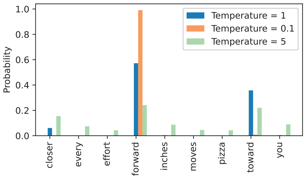
\(T = 1\) divides the logits by 1 and leaves the original probability scores unchanged.
"forward"is selected about 60% of the time.Sampling at \(T = 1\) is the same as not applying temperature scaling at all.
\(T < 1\) amplifies the differences between logits, giving a sharper distribution. At \(T = 0.1\),
multinomialselects"forward"almost 100% of the time, approaching the behavior ofargmax.This is why very low temperature is the practical equivalent of greedy decoding.
\(T > 1\) flattens the distribution toward uniform. At \(T = 5\), less likely tokens are selected more often, which adds variety and also produces nonsensical text such as
every effort moves you pizzaabout 4% of the time.The failure mode is not a rare accident; it is the direct consequence of giving implausible tokens non-negligible probability.
Learning outcomes
- temperature-scaling Replace greedy decoding with multinomial sampling controlled by a temperature.
Concepts
- greedy-decoding
torch.argmaxalways returns the same continuation for a given start context, which for an overfitted model is a memorized passage - temperature-scaling dividing the logits by \(T\) before
softmaxsharpens the distribution for \(T < 1\) and flattens it for \(T > 1\), with \(T = 1\) leaving it unchanged
Top-k sampling and a better generate
Flattening the distribution makes grammatically incorrect or completely nonsensical outputs such as every effort moves you pizza reachable. Top-k sampling removes them by restricting the sampled tokens to the \(k\) most likely ones and excluding all others from the selection process.
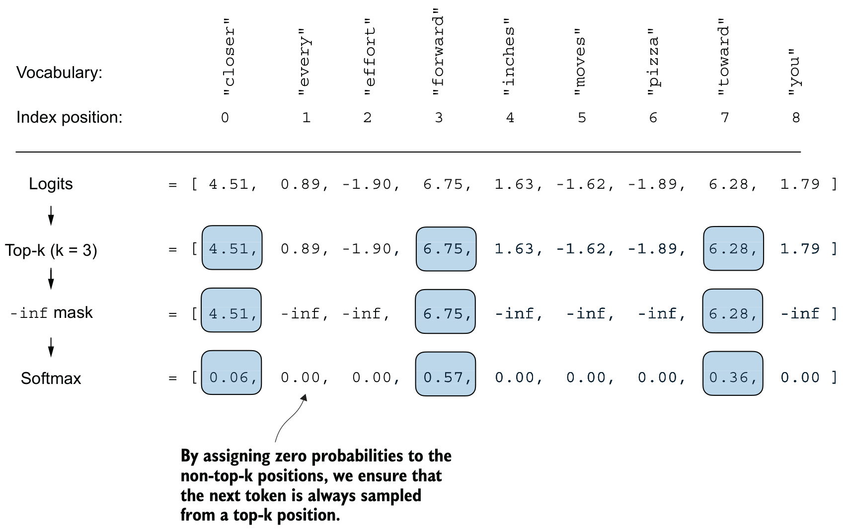
-inf, and the softmax then assigns probability 0 to every non-top-k token.On the nine-token example:
top_k = 3
top_logits, top_pos = torch.topk(next_token_logits, top_k)
This gives Top logits: tensor([6.7500, 6.2800, 4.5100]) and Top positions: tensor([3, 7, 0]), in descending order. Every logit below the smallest of those three is replaced with negative infinity:
new_logits = torch.where(
    condition=next_token_logits < top_logits[-1],
    input=torch.tensor(float('-inf')),
    other=next_token_logits
)
The result is tensor([4.5100, -inf, -inf, 6.7500, -inf, -inf, -inf, 6.2800, -inf]), and torch.softmax(new_logits, dim=0) gives tensor([0.0615, 0.0000, 0.0000, 0.5775, 0.0000, 0.0000, 0.0000, 0.3610, 0.0000]). The masked tokens receive probability exactly 0, so they can never be sampled, and the three survivors are renormalized to sum to 1. This is the same masking device used by the causal attention module.
One function for every control
Listing 5.4 folds context cropping, top-\(k\) filtering, temperature scaling and early stopping into a replacement for generate_text_simple:
def generate(model, idx, max_new_tokens, context_size,
             temperature=0.0, top_k=None, eos_id=None):
    for _ in range(max_new_tokens):
        idx_cond = idx[:, -context_size:]
        with torch.no_grad():
            logits = model(idx_cond)
        logits = logits[:, -1, :]
        if top_k is not None:
            top_logits, _ = torch.topk(logits, top_k)
            min_val = top_logits[:, -1]
            logits = torch.where(
                logits < min_val,
                torch.tensor(float('-inf')).to(logits.device),
                logits
            )
        if temperature > 0.0:
            logits = logits / temperature
            probs = torch.softmax(logits, dim=-1)
            idx_next = torch.multinomial(probs, num_samples=1)
        else:
            idx_next = torch.argmax(logits, dim=-1, keepdim=True)
        if idx_next == eos_id:
            break
        idx = torch.cat((idx, idx_next), dim=1)
    return idx
The order of the two controls is what makes them compose: top-\(k\) decides which tokens are candidates, and the temperature then decides how evenly to sample among the survivors. The temperature > 0.0 test is what preserves greedy decoding — at temperature=0.0 the else branch runs torch.argmax and the function reproduces generate_text_simple.
Called on the overfitted model with max_new_tokens=15, top_k=25 and temperature=1.4, the output is
 Every effort moves you stand to work on surprise, a one of us had gone
 with random-
which is not the memorized passage the same start context produced under greedy decoding.
Learning outcomes
- top-k-sampling-and-the-generate-function Restrict sampling to the top-k candidates and combine the decoding controls into one generate function.
- temperature-scaling Replace greedy decoding with multinomial sampling controlled by a temperature.
Concepts
- top-k-sampling
torch.topkselects the \(k\) largest logits andtorch.wheresets the rest to-inf, so the softmax gives every excluded token probability 0 - temperature-scaling inside
generatethe logits are divided by the temperature after top-\(k\) masking, and only when the temperature exceeds 0 - greedy-decoding
generatefalls back totorch.argmaxwhen the temperature is 0.0, which recovers the deterministic behavior ofgenerate_text_simple
Saving and loading checkpoints
Pretraining is computationally expensive even at this scale, so the trained weights are worth keeping rather than recomputing in each new session. The recommended way is to save the model’s state_dict, a dictionary mapping each layer to its parameters:
torch.save(model.state_dict(), "model.pth")The .pth extension is a convention for PyTorch files, not a requirement. Restoring it requires an architecture to restore into:
model = GPTModel(GPT_CONFIG_124M)
model.load_state_dict(torch.load("model.pth", map_location=device))
model.eval()
model.eval() matters here. Dropout randomly drops a layer’s neurons during training to prevent overfitting; during inference there is no reason to drop any of the information the network has learned, and evaluation mode disables those layers.
What the weights alone leave out
AdamW stores additional parameters for each model weight, using historical data to adjust the learning rate for each parameter dynamically. Restoring only model.state_dict() discards those running estimates. The optimizer then resets, and the model may learn suboptimally or even fail to converge properly, which means it will lose the ability to generate coherent text. A checkpoint intended for resumption holds both state dictionaries:
torch.save({
    "model_state_dict": model.state_dict(),
    "optimizer_state_dict": optimizer.state_dict(),
    },
    "model_and_optimizer.pth"
)
Both are restored the same way, and the model is returned to training mode rather than evaluation mode:
checkpoint = torch.load("model_and_optimizer.pth", map_location=device)
model = GPTModel(GPT_CONFIG_124M)
model.load_state_dict(checkpoint["model_state_dict"])
optimizer = torch.optim.AdamW(model.parameters(), lr=5e-4, weight_decay=0.1)
optimizer.load_state_dict(checkpoint["optimizer_state_dict"])
model.train();After saving the weights, load the model and optimizer in a new Python session or Jupyter notebook file and continue pretraining it for one more epoch using the train_model_simple function.
Loading a state_dict into an architecture that was constructed separately is the same mechanism the next section applies to weights that were never produced by this code at all.
Learning outcomes
- checkpointing-model-and-optimizer Save and restore model weights together with optimizer state.
Concepts
- checkpoint-saving-loading
torch.savewrites astate_dictandload_state_dictreads it back; a resumable checkpoint holds the model’s and the optimizer’s dictionaries together - adamw-optimizer its per-parameter historical estimates are part of the training state, so a checkpoint without them restarts the optimizer from cold
Loading OpenAI pretrained weights
OpenAI openly shared the weights of their GPT-2 models, which removes the need to invest tens to hundreds of thousands of dollars in retraining a model of that size on a large corpus. The weights were originally saved via TensorFlow, so TensorFlow and a progress-bar tool are installed first:
pip install tensorflow>=2.15.0 tqdm>=4.66The download code is fetched as a module rather than reproduced, and download_and_load_gpt2 returns the architecture settings and the weight tensors:
from gpt_download import download_and_load_gpt2
settings, params = download_and_load_gpt2(
    model_size="124M", models_dir="gpt2"
)
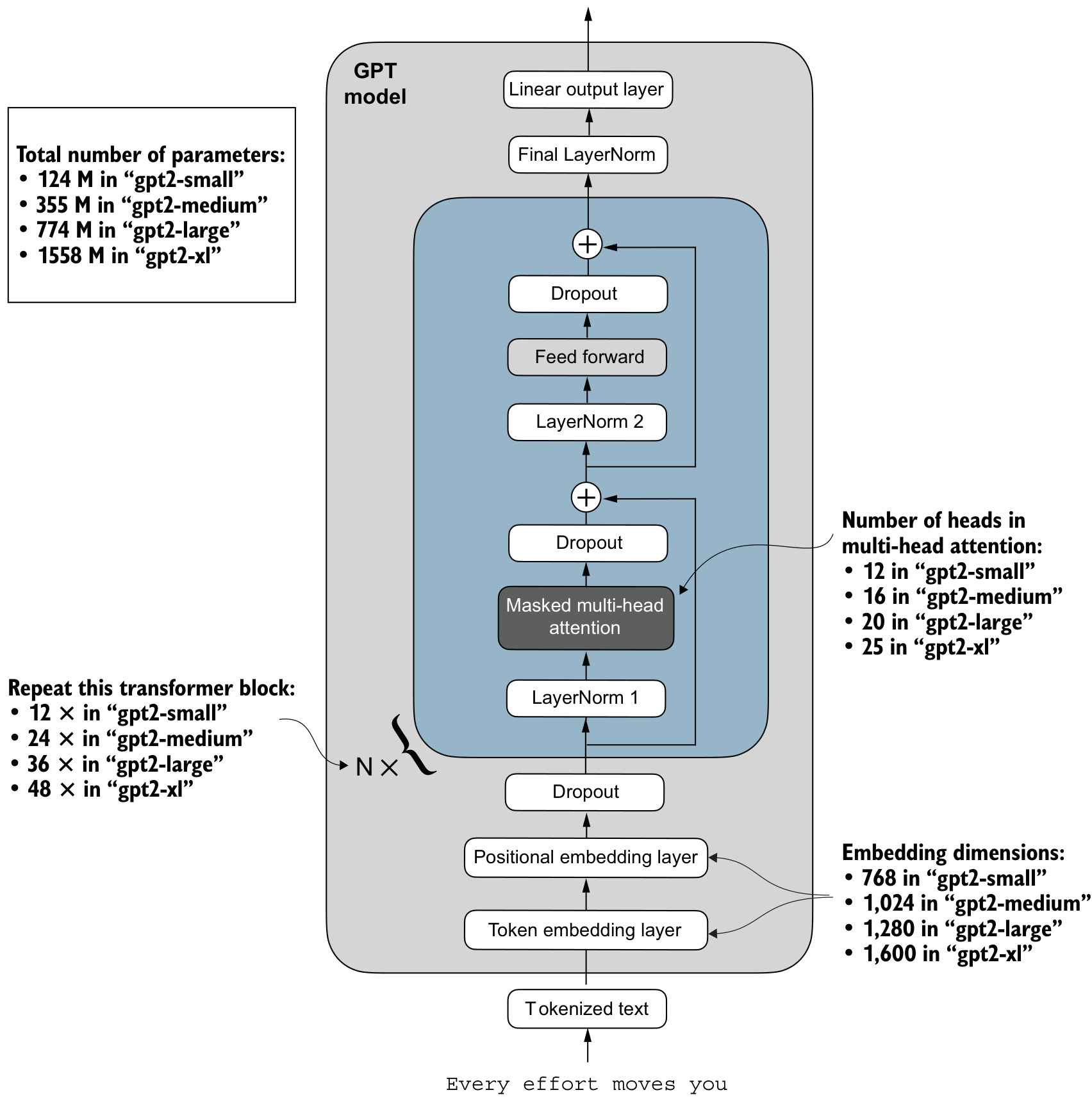
settings is {'n_vocab': 50257, 'n_ctx': 1024, 'n_embd': 768, 'n_head': 12, 'n_layer': 12} and params has keys dict_keys(['blocks', 'b', 'g', 'wpe', 'wte']). The token embedding tensor params["wte"] has dimensions (50257, 768).
Matching the configuration
model_configs = {
    "gpt2-small (124M)": {"emb_dim": 768, "n_layers": 12, "n_heads": 12},
    "gpt2-medium (355M)": {"emb_dim": 1024, "n_layers": 24, "n_heads": 16},
    "gpt2-large (774M)": {"emb_dim": 1280, "n_layers": 36, "n_heads": 20},
    "gpt2-xl (1558M)": {"emb_dim": 1600, "n_layers": 48, "n_heads": 25},
}
Two further adjustments are required. The context length was reduced to 256 for laptop training, but the original GPT-2 models were trained with a 1,024-token length, so NEW_CONFIG.update({"context_length": 1024}). And OpenAI used bias vectors in the query, key and value linear layers of the multi-head attention module. Bias vectors are not commonly used in LLMs anymore, as they don’t improve the modeling performance and are thus unnecessary; matching the released weights nevertheless requires NEW_CONFIG.update({"qkv_bias": True}).
The mapping
A shape check guards every assignment:
def assign(left, right):
    if left.shape != right.shape:
        raise ValueError(f"Shape mismatch. Left: {left.shape}, "
                         "Right: {right.shape}"
        )
    return torch.nn.Parameter(torch.tensor(right))
Listing 5.5 walks the transformer blocks. The combined attention tensor is split into three:
def load_weights_into_gpt(gpt, params):
    gpt.pos_emb.weight = assign(gpt.pos_emb.weight, params['wpe'])
    gpt.tok_emb.weight = assign(gpt.tok_emb.weight, params['wte'])

    for b in range(len(params["blocks"])):
        q_w, k_w, v_w = np.split(
            (params["blocks"][b]["attn"]["c_attn"])["w"], 3, axis=-1)
        gpt.trf_blocks[b].att.W_query.weight = assign(
            gpt.trf_blocks[b].att.W_query.weight, q_w.T)
The same np.split is applied to the bias tensor, and the remaining assignments cover att.out_proj, the two ff.layers weights and biases, and the norm1 and norm2 scales and shifts, each transposed where OpenAI’s layout differs. The function ends with:
    gpt.final_norm.scale = assign(gpt.final_norm.scale, params["g"])
    gpt.final_norm.shift = assign(gpt.final_norm.shift, params["b"])
    gpt.out_head.weight = assign(gpt.out_head.weight, params["wte"])
That last line is weight tying: the original GPT-2 model reused the token embedding weights in the output layer to reduce the total number of parameters, so params["wte"] is assigned twice — once to tok_emb and once to out_head.
Developing load_weights_into_gpt took a lot of guesswork, since OpenAI used a different naming convention. The assign function is what makes a mistake detectable: it raises on any dimension mismatch, and an error that slipped past it would show up as a model unable to produce coherent text.
Verification
torch.manual_seed(123)
token_ids = generate(
    model=gpt,
    idx=text_to_token_ids("Every effort moves you", tokenizer).to(device),
    max_new_tokens=25,
    context_size=NEW_CONFIG["context_length"],
    top_k=50,
    temperature=1.5
)
The output is
 Every effort moves you toward finding an ideal new way to practice
    something!
What makes us want to be on top of that?
Coherent English is the confirmation that the mapping is correct, because a tiny mistake in this process would cause the model to fail.
Learning outcomes
- loading-openai-gpt2-weights Map OpenAI’s released GPT-2 weights into your own PyTorch implementation.
- checkpointing-model-and-optimizer Save and restore model weights together with optimizer state.
- top-k-sampling-and-the-generate-function Restrict sampling to the top-k candidates and combine the decoding controls into one generate function.
Concepts
- weight-tying GPT-2 assigns
params["wte"]to both the token embedding layer andout_head.weight, so one tensor serves two positions - checkpoint-saving-loading
load_weights_into_gpttransfers externally released tensors into the modules of aGPTModelinstance, withassignverifying each shape
A pretrained model in hand
When LLMs generate text, they output one token at a time.
Every measurement and every decoding control in this unit acts on the distribution over the single next token.
Cross entropy loss and its exponential, perplexity, gauge the quality of text generated by an LLM during training.
A loss of 10.7940 corresponds to a perplexity of 48,725.8203, which is the effective vocabulary size an untrained model is undecided among.
Pretraining an LLM involves changing its weights to minimize the training loss, and the loop itself is a standard deep learning procedure using cross entropy loss and the AdamW optimizer.
Nothing in
train_model_simpleis specific to language modeling apart from the loss function it calls.Probabilistic sampling and temperature scaling influence the diversity and coherence of the generated text; top-\(k\) filtering removes the implausible tokens a high temperature would otherwise admit.
Training loss of 0.391 against a validation loss of 6.452 on 5,145 tokens is memorization, and decoding — not the weights — is what breaks the model out of reciting.
Pretraining an LLM on a large text corpus is time- and resource-intensive, so openly available weights are an alternative to pretraining the model on a large dataset oneself.
The implementation of the previous unit accepts OpenAI’s GPT-2 tensors without modification, which is evidence that it is the same model and not an approximation of one.
The pretrained GPT-2 is a general next-token predictor: it completes text, and it neither answers questions nor assigns labels. 6 Fine-tuning for classification specializes it, replacing the 50,257-unit vocabulary head with a Linear(768, 2) classification head, freezing the backbone apart from the last transformer block and the final LayerNorm, and reading the class logits from outputs[:, -1, :] — the only position that causal masking allows to see the whole input. The cross entropy loss, the AdamW loop and the checkpointing written here carry over unchanged; only the head and the targets differ.
Learning outcomes
- cross-entropy-loss-and-perplexity Compute the text generation loss from logits and interpret it as perplexity.
- pretraining-loop-with-adamw Write a complete pretraining loop that optimizes an LLM with AdamW.
- diagnosing-overfitting Read training and validation loss curves to recognize memorization.
- loading-openai-gpt2-weights Map OpenAI’s released GPT-2 weights into your own PyTorch implementation.
- checkpointing-model-and-optimizer Save and restore model weights together with optimizer state.
References
- Building a Large Language Model (from scratch), Sebastian Raschka, 2024, Manning Books — Link — Page 150-190