5 Pretraining on unlabeled data

Language Models · v1.0.0

2026-08-25 14:44:41

From a random model to a trained one

Where we left off

In 4 Implementing a GPT model from scratch to generate text we assembled a complete GPTModel and a greedy generation loop.

The architecture was finished.
The output was not — every weight was random, so the model emitted noise.

What was missing

a measure of error — cross entropy loss and perplexity
an optimization loop — AdamW, backpropagation, train/validation split
better decoding — temperature and top-$k$ sampling
persistence — checkpoints, and OpenAI’s own GPT-2 weights

This is stage 2 of building an LLM: pretraining.

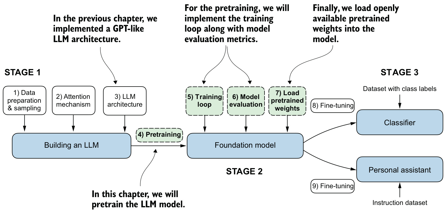
The three main stages of coding an LLM. This unit is stage 2.

Our approach

We train on a small public-domain story so every experiment runs on a laptop in minutes.

That choice has a consequence we will see plainly: the model memorises rather than generalises.
We then sidestep the compute problem entirely by importing weights OpenAI trained for us.

From logits to a loss

Generating text, again

The model is the one built previously, with its context length shortened from 1,024 to 256 tokens so training fits on a laptop.

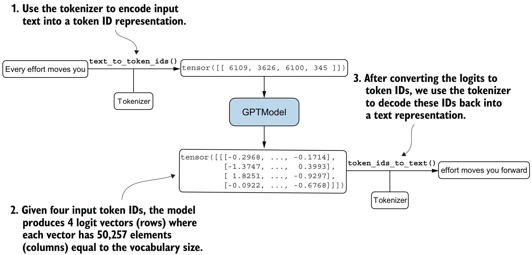
Generating text encodes text into token IDs, which the LLM processes into logit vectors. The logits are converted back into token IDs and detokenized.

Gibberish needs a number

Running the untrained model on "Every effort moves you" with greedy decoding — always taking the highest-probability token — produces gibberish.

The model has not been trained.
To define what “coherent” means, we need a number.

The manual derivation

Take a batch of tokenized inputs and targets, where each target is the input shifted one position forward.

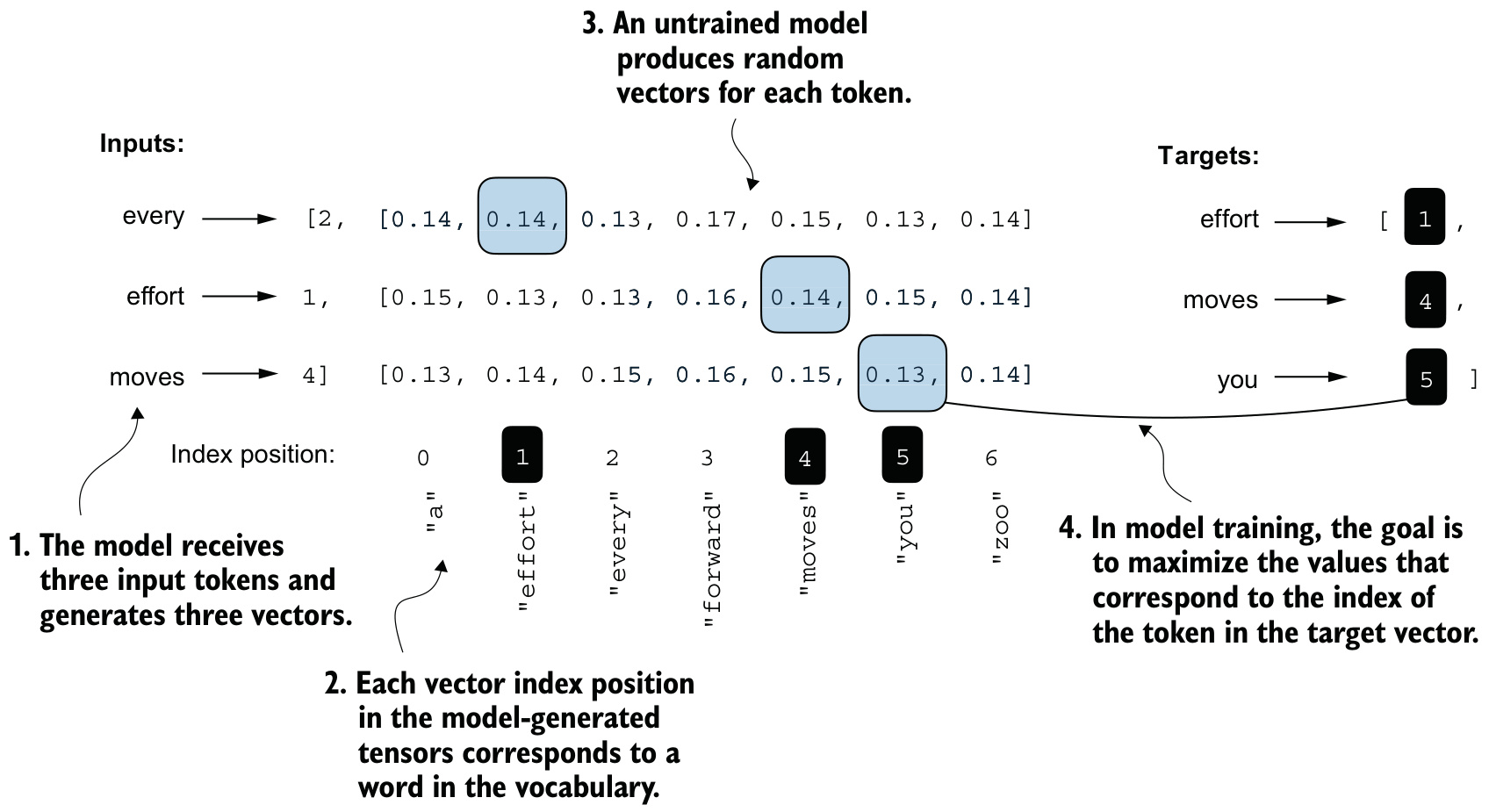
Before training, the model produces random next-token probability vectors. Training aims to maximise the probability values at the highlighted target token IDs.

Three conceptual steps

target_probas = probas[batch, positions, target_ids]   # probability assigned to each true next token
neg_avg_log = -mean(log(target_probas))                 # negative average log-likelihood

Before training, target_probas is close to $1/|V|$ for a vocabulary of size $|V|$.

Training is exactly the process of pushing these probabilities up.

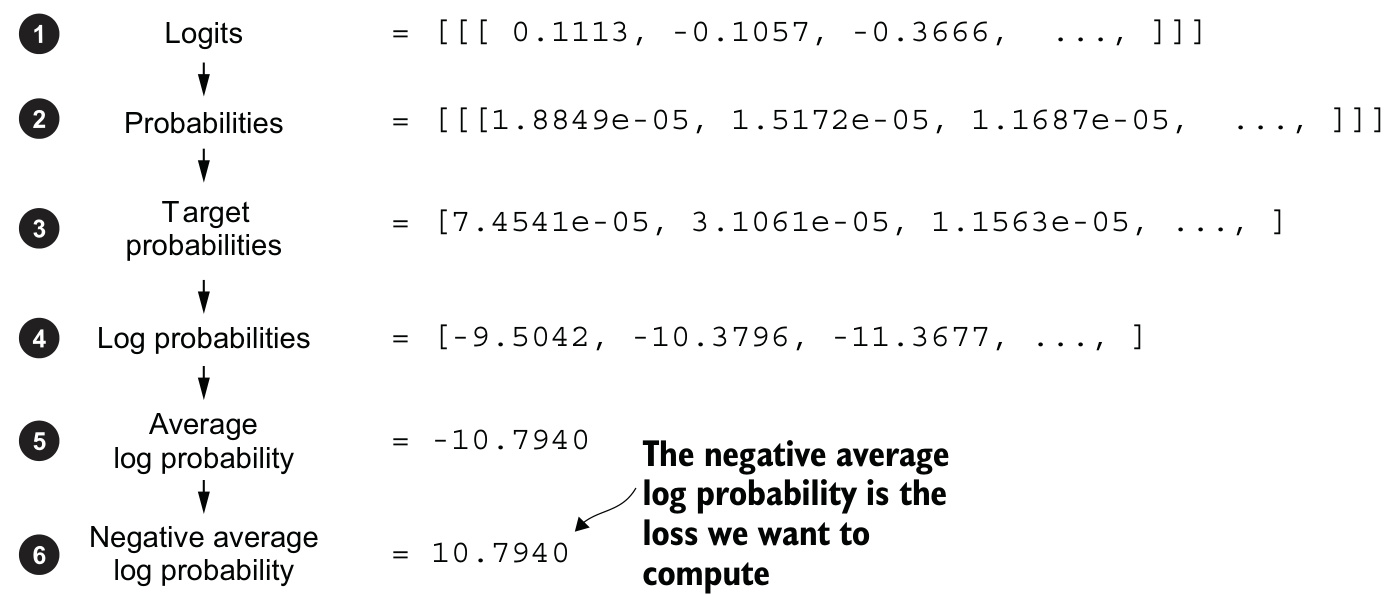
Steps to obtain the token probabilities at the target positions, then transform them by a logarithm, average, and negate.

Why the logarithm

Why the logarithm

Working with logarithms of probability scores is more manageable in mathematical optimization than handling the scores directly.

The deep learning convention is not to push the average log probability up toward $0$, but to bring the negative average log probability down toward $0$.

The library version

This quantity — cross entropy loss — is exactly what PyTorch’s cross_entropy computes in one call from the raw logits and target token IDs.

\[\mathcal{L} = -\frac{1}{N}\sum_{i=1}^{N} \log p(y_i \mid x_i)\]

No need to write the softmax, indexing, or logarithm by hand.

Perplexity

Perplexity is the exponential of the loss:

\[\text{perplexity} = e^{\mathcal{L}}\]

It reads as the effective vocabulary size the model is undecided among.

Training and validation losses

Measuring a whole dataset

A loss on a couple of hand-picked sentences is not a measurement of a model.

Corpus: “The Verdict”, a short story by Edith Wharton.
Public domain, about 5,145 tokens — every experiment runs on a laptop in minutes.

The cost of pretraining LLMs

Llama 2 7B required 184,320 GPU hours on A100 GPUs over 2 trillion tokens — roughly $690,000. Our corpus has 5,145 tokens.

The split and the loaders

The corpus is split 90/10 into training and validation text, each fed through the sliding-window loader with window length and stride equal to the context length.

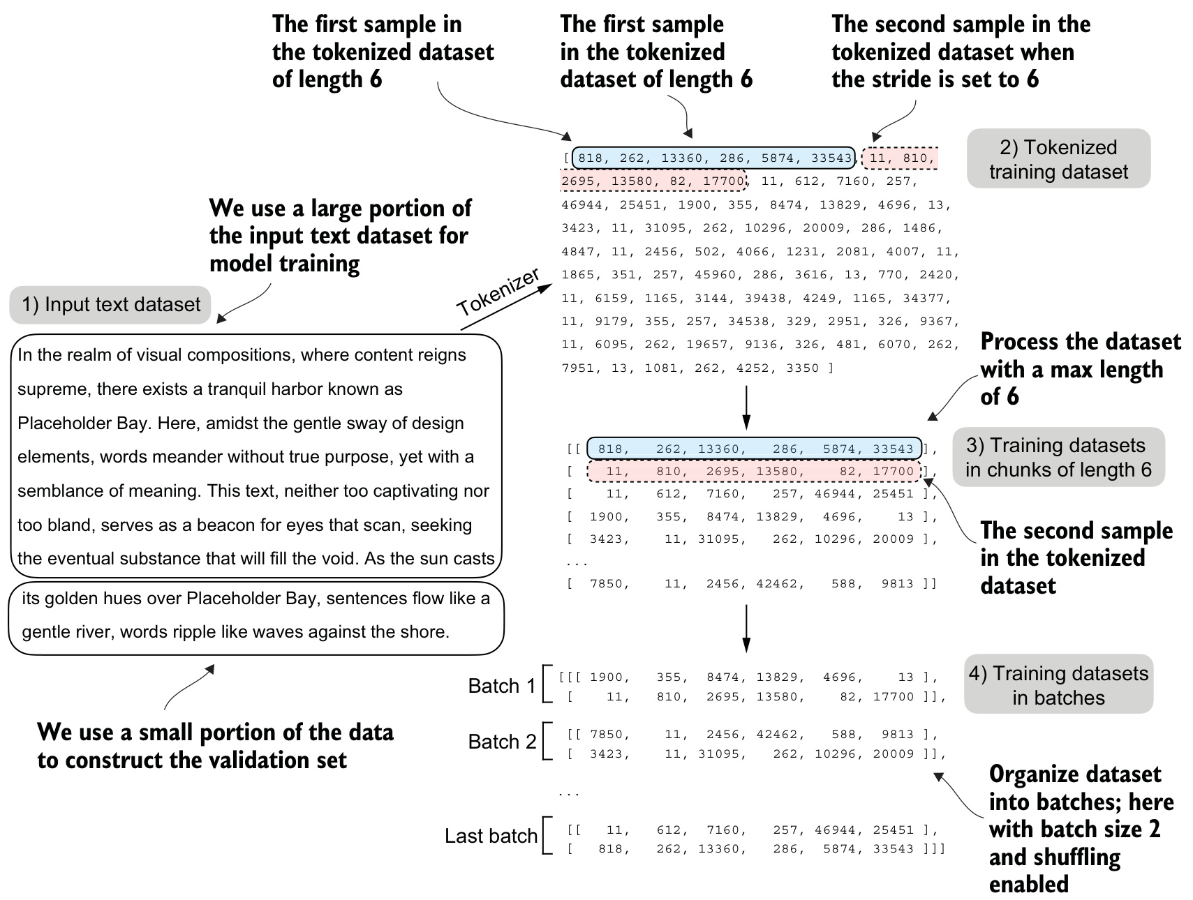
The input text is split into training and validation portions, tokenized, divided into fixed-length chunks, shuffled and organised into batches.

Two functions

def batch_loss(model, inputs, targets):
    return cross_entropy(model(inputs), targets)

def loader_loss(model, loader, num_batches=None):
    return mean(batch_loss(model, x, y) for x, y in first(loader, num_batches))

batch_loss measures a single batch.
loader_loss averages over a loader, optionally over just a few batches for a cheap estimate.

Before any training

Applied to both loaders before training, both losses come out close to:

\[\log |V| \approx 10.98\]

This is the loss of a model that has learned nothing.
The loss approaches $0$ if the model learns to reproduce the data exactly.

The pretraining loop

Ordinary deep learning practice

For each epoch: iterate over training batches, compute the loss, backpropagate, and step the optimizer.

Periodically evaluate both losses with dropout and gradient tracking disabled.
Print a sample continuation so progress is visible as text, not just numbers.

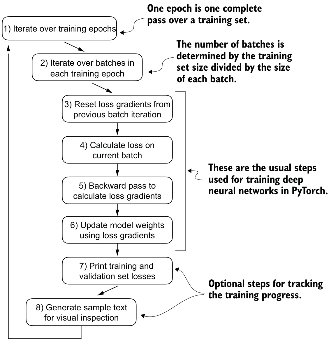
A typical PyTorch training loop iterates over the batches of the training set for several epochs, computing the loss, deriving gradients, and updating the weights.

The loop

def pretrain(model, train_loader, val_loader, optimizer, num_epochs):
    for epoch in range(num_epochs):
        for inputs, targets in train_loader:
            loss = batch_loss(model, inputs, targets)
            loss.backward()
            optimizer.step()
            optimizer.zero_grad()
            if time_to_evaluate():
                log(loader_loss(model, train_loader), loader_loss(model, val_loader))
        sample_and_print(model, prompt="Every effort moves you")

AdamW

AdamW

AdamW is a variant of Adam that improves the weight decay approach, which aims to minimise model complexity and prevent overfitting by penalising larger weights.

The adjustment allows more effective regularization and better generalization — AdamW is the standard choice for LLM training.

The run

Training this configuration for 10 epochs on “The Verdict” takes about five minutes on a laptop.

Training loss falls from around 9.8 to 0.4.
Early samples are pure repetition; by the end the model writes grammatically correct English.
The validation loss falls with the training loss at first, then stalls well above it.

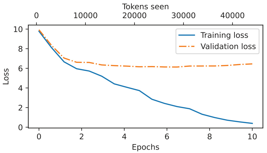
Both losses drop sharply at first. Past epoch 2 the training loss keeps falling while the validation loss stagnates — the model is overfitting.

Reading the curves

The divergence past epoch 2, and the size of the gap, tell us the model is overfitting.

Confirmed directly: generated sentences can be found verbatim in the source text.
The model has memorised, not generalised.

Expected: the dataset is small and we trained for multiple epochs. In practice, train on a much larger dataset for only one epoch.

Key ideas

The LLM training loop is ordinary deep learning: zero gradients, compute loss, backpropagate, step.
AdamW is chosen for its decoupled weight decay, not for anything LLM-specific.
A falling training loss alongside a flat validation loss is the signature of memorization.
Verbatim recall is a property of the corpus size, not a defect of the code.

Temperature scaling

The decoding problem

The trained model still disappoints, and the reason is not the weights — it is the decoding.

Greedy decoding (argmax) is deterministic.
The same prompt always produces the identical continuation.
On a small corpus, that continuation is often a memorised passage.

Probabilistic sampling

Replace argmax with sampling in proportion to each token’s probability — drawing from the softmax distribution rather than taking its peak.

The most likely token still wins most draws.
Occasionally another plausible token is chosen instead.
Low-probability tokens are drawn rarely, if ever.

The temperature

Temperature scaling divides the logits by a number $T > 0$ before the softmax:

\[p_i = \frac{\exp(z_i / T)}{\sum_j \exp(z_j / T)}\]

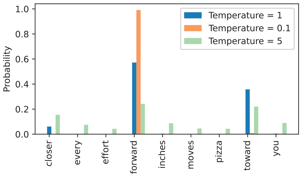
$T = 1$: same as no scaling — original softmax probabilities.
$T < 1$: sharpens the distribution, approaching argmax as $T \to 0$.
$T > 1$: flattens it — more variety, but also more nonsense.

Seeing the effect

A temperature of 1 gives the unscaled scores. Lowering it to 0.1 sharpens the distribution; raising it to 5 makes it more uniform.

Creativity and coherence pull in opposite directions, and the temperature is the dial between them.

Top-k sampling and a better generate

Removing the implausible tail

Higher temperatures explore less likely — and potentially more interesting — paths, but at the cost of sometimes producing nonsensical output.

Top-$k$ sampling restricts the candidate set before sampling.

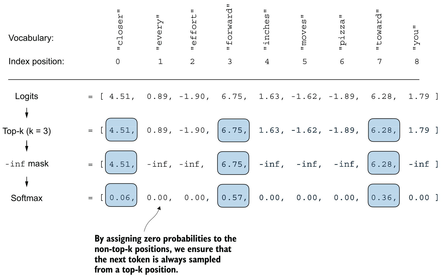
With $k = 3$ we keep the three largest logits, mask the rest with $-\infty$, and apply the softmax. Every non-top-$k$ token then has probability 0.

The masking trick

Only the $k$ largest logits survive; every other logit is set to $-\infty$, so after softmax those tokens receive probability exactly zero — since $e^{-\infty} = 0$.

The same masking trick used by causal attention.
Top-$k$ decides which tokens are candidates.
Temperature decides how evenly to sample among them.

One generate function $^1/_2$

def generate(model, idx, max_new_tokens, temperature=0.0, top_k=None, eos_id=None):
    for _ in range(max_new_tokens):
        logits = last_position_logits(model, idx)
        if top_k is not None:
            logits = mask_below_top_k(logits, top_k)

Each step optionally masks to the top-$k$ logits before deciding how to pick the next token.

One generate function $^2/_2$

        if temperature > 0.0:
            next_id = sample(softmax(logits / temperature))
        else:
            next_id = argmax(logits)
        if next_id == eos_id:
            break
        idx = append(idx, next_id)
    return idx

Greedy decoding is the special case temperature = 0.0 — the old behaviour is subsumed, not discarded.

Saving and loading checkpoints

Why persist

Pretraining is computationally expensive even at this scale, so the model must be saved rather than retrained every time it is needed.

Save the model’s parameter dictionary — a mapping from each layer to its weight tensors.
To reload: construct a fresh architecture, then assign the saved parameters into it.

Why switch to evaluation mode after loading

Dropout randomly drops neurons during training to prevent overfitting. At inference we do not want to discard learned information, so the reloaded model is switched to evaluation mode, which disables dropout.

The optimizer state matters too

Adaptive optimizers such as AdamW store per-parameter statistics used to adjust the learning rate for each weight dynamically.

Without that history the optimizer resets.
The model may learn suboptimally or fail to converge if training resumes.

A checkpoint intended for resuming training holds both the model’s and the optimizer’s state.

The shape of the operation

Notice the pattern: construct an architecture, then assign parameters into it by name.

That is exactly the mechanism the next section uses, with OpenAI supplying the parameters instead of our own training run.

Loading OpenAI pretrained weights

Borrowing instead of training

OpenAI openly released the weights of their GPT-2 models.

Eliminates the need to invest tens to hundreds of thousands of dollars retraining ourselves.
The pretrained parameters can simply be poured into our own architecture, provided the shapes match.

Four sizes, one architecture

OpenAI released four sizes of GPT-2. The core architecture is identical across them; only the embedding size and the number of repeated components differ.

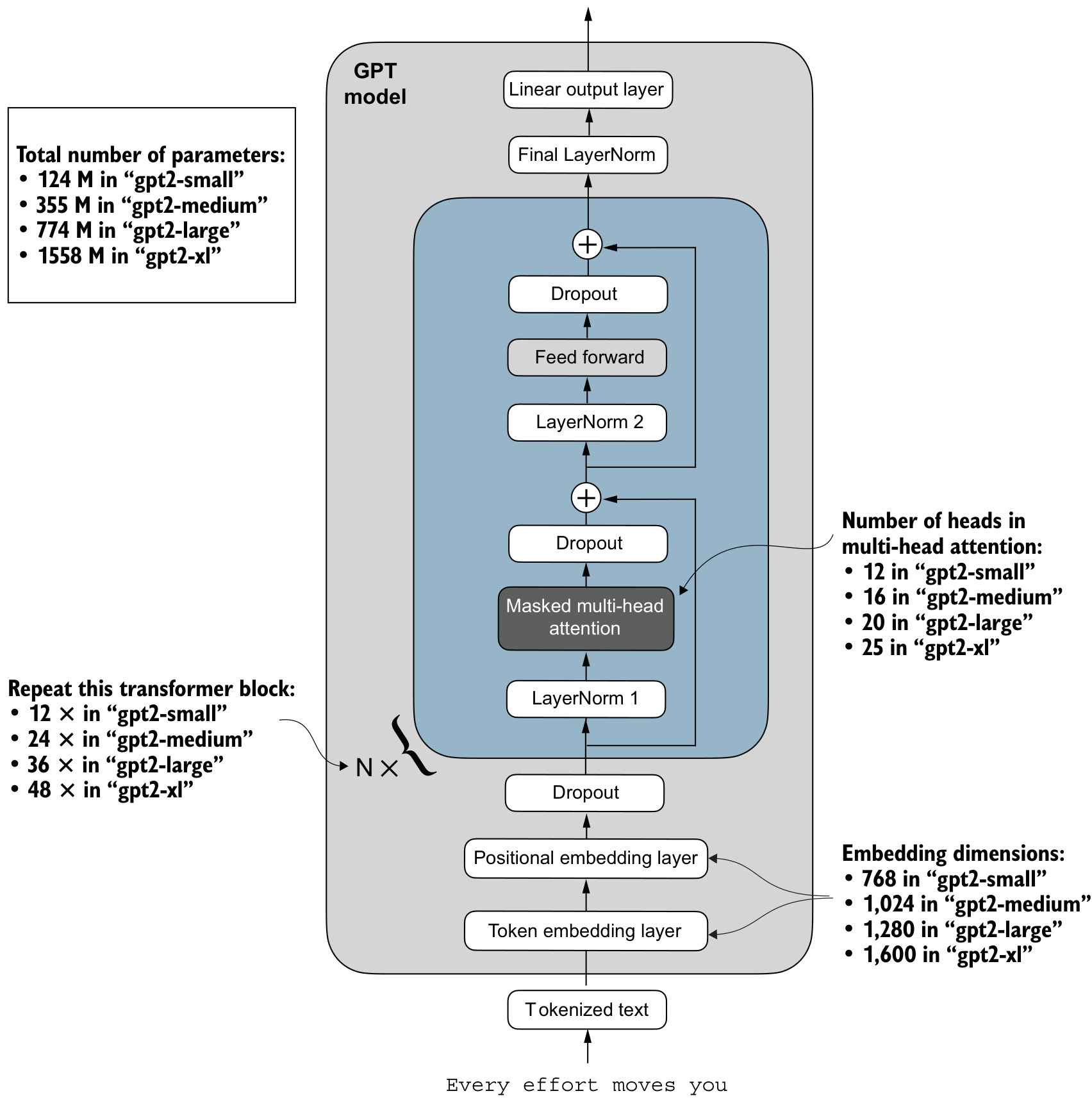
GPT-2 ranges from 124 million to 1,558 million parameters. The architecture is the same; the embedding size and the repetition counts change.

Configuring our model to match

To accept OpenAI’s weights, our configuration must match theirs:

context length returns to 1,024 (256 was a laptop concession)
query/key/value bias vectors enabled — OpenAI’s implementation used them, even though modern LLMs typically don’t

The mapping

Loading is a walk over every tensor in OpenAI’s checkpoint, assigning each into the corresponding parameter of our model, with a shape check at every step.

def load_weights_into_gpt(gpt, params):
    assign(gpt.pos_emb, params.wpe)
    assign(gpt.tok_emb, params.wte)
    for block, block_params in zip(gpt.trf_blocks, params.blocks):
        assign_attention_weights(block.att, block_params.attn)   # split combined QKV, transpose
        assign_feedforward_weights(block.ff, block_params.mlp)
        assign_layernorm_weights(block.norm1, block.norm2, block_params)
    assign(gpt.final_norm, params.final_ln)
    assign(gpt.out_head, params.wte)   # weight tying: reuse the token embedding matrix

Three details worth naming

The combined QKV projection is split. OpenAI stored query, key and value weights as one tensor, divided into three equal parts.
Weights are transposed. TensorFlow’s layout is the transpose of PyTorch’s.
The output head reuses the token embedding matrix. This is weight tying: GPT-2 uses the same tensor as both the input embedding and the final output projection.

Verification

With the weights loaded, generating from "Every effort moves you" with temperature and top-$k$ sampling produces coherent English.

Proof that both the architecture and the weight assignment are correct — a single mismatched tensor would corrupt the output.

A pretrained model in hand

Summary $^1/_2$

Cross entropy loss and perplexity give a quantifiable measure of an LLM’s next-token predictions.
The training loop for LLMs is a standard deep learning procedure using cross entropy loss and AdamW.
Training loss falling while validation loss stagnates means the model is memorising the corpus.
Probabilistic sampling and temperature scaling influence the diversity and coherence of generated text.

Summary $^2/_2$

Top-$k$ filtering makes high temperatures usable by removing the implausible tail.
A checkpoint must hold the optimizer state as well as the weights.
Pretraining on a large corpus is time- and resource-intensive, so we can load openly available weights instead.

Where this leaves us

A pretrained GPT-2 is a general next-token predictor.

It completes text.
It does not answer questions or label anything.

Stage 3 of building an LLM is adapting it.

Where next

The next unit, 6 Fine-tuning for classification, takes this pretrained model and specialises it to predict fixed categories.

The 50,257-unit vocabulary head is replaced with a small class-sized linear layer.
Most of the backbone is frozen.
Classification logits are read from the last token position.

The loss function, training loop and checkpointing learned here carry over unchanged — only the head and the targets differ.