Lecture notes — 6 Fine-tuning for classification
ver. 1.2.0, 6_fine_tuning_for_classification
← 6 Fine-tuning for classification
ver. 1.2.0 · 2026-09-02 16:27:04
Where this fits
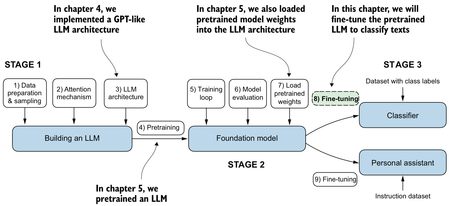
The previous unit, 5 Pretraining on unlabeled data, ended with OpenAI’s GPT-2 124M weights mapped into a GPTModel written from scratch, a checkpointing routine, and a generate function that produces coherent English. That model predicts the next token and nothing else. Stage 3 of building an LLM is adaptation, and this unit performs the narrow version of it: a pretrained GPT-2 is turned into a binary classifier for text messages, trained on 1,494 labeled examples.
Four things change; the rest is carried over unaltered.
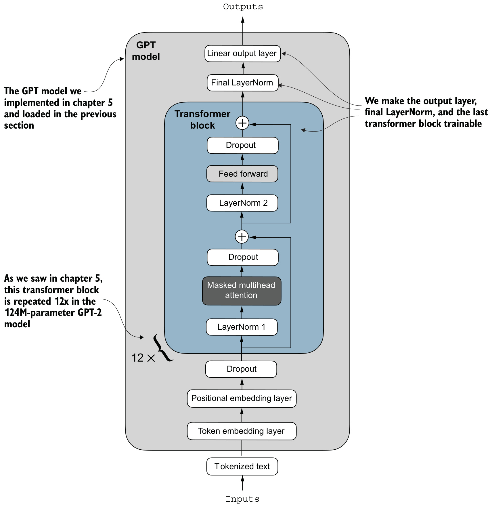
- Keep the backbone. The embeddings and eleven of the twelve transformer blocks stay frozen, so the general language representations obtained by pretraining are preserved.
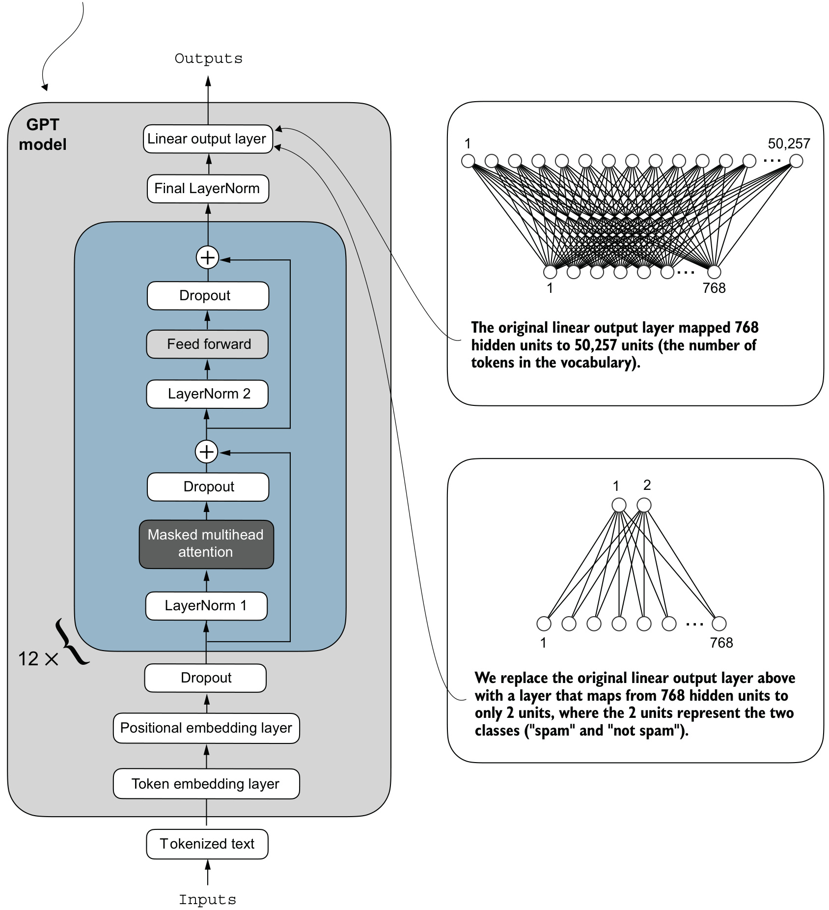
- Change the head. The \(768 \rightarrow 50257\) vocabulary projection becomes \(768 \rightarrow 2\).
- Change the position read out. The classification logits come from the final token position, not from every position.
- Keep the machinery. The AdamW loop,
torch.nn.functional.cross_entropy, the loader-averaged loss andtorch.saveon astate_dictall reappear here.
Learning outcomes
choosing-a-fine-tuning-approach— Choose between classification and instruction fine-tuning for a given task.preparing-a-balanced-labeled-dataset— Download, balance and split a labeled text dataset for supervised fine-tuning.padded-datasets-and-loaders— Build a PyTorch Dataset that tokenizes and pads variable-length texts to a uniform length.freezing-a-pretrained-backbone— Load pretrained GPT-2 weights and freeze the parameters you do not want to train.replacing-the-output-head— Swap the vocabulary projection for a class-sized classification head.last-token-classification-logits— Take the classification decision from the final token position.classification-loss-and-accuracy— Compute classification cross-entropy loss and accuracy over a data loader.running-the-supervised-fine-tuning— Fine-tune the adapted model with AdamW and read its loss and accuracy curves.deploying-the-classifier— Use and persist the fine-tuned classifier on new text.
Concepts introduced
- Classification fine-tuning — training a pretrained language model on labeled data so that it maps an input to one member of a fixed, predefined set of class labels.
- Instruction fine-tuning — training a language model on instruction–response pairs so that it executes tasks described in natural language prompts.
- Dataset undersampling — reducing the majority class to the size of the minority class by random sampling, so that class frequencies are equal.
- Sequence padding and truncation — standardizing variable-length token sequences to one length by cutting those that exceed it and appending a designated padding token to those that fall short.
- Classification head — a linear layer that replaces the vocabulary projection and maps the embedding dimension to the number of target classes.
- Selective parameter freezing — setting
requires_grad = Falseon most pretrained parameters and leaving only a chosen few trainable. - Last-token prediction pooling — taking the output vector at the final sequence position as the representation of the whole input, and computing loss and predictions from it alone.
Which kind of fine-tuning
Two approaches dominate the adaptation of language models. Instruction fine-tuning trains a language model on a set of tasks using specific instructions, to improve its ability to understand and execute tasks described in natural language prompts. Classification fine-tuning trains the model to recognize a specific set of class labels, such as “spam” and “not spam”.
Classification tasks are not confined to language models. Raschka’s examples extend to identifying different species of plants from images, categorizing news articles into topics like sports, politics, and technology, and distinguishing between benign and malignant tumors in medical imaging.
The key point is that a classification fine-tuned model is restricted to predicting classes it has encountered during its training. It can determine whether something is “spam” or “not spam”, but it cannot say anything else about the input text. An instruction fine-tuned model, by contrast, can undertake a broader range of tasks — asked “Translate into German: ‘The quick brown fox jumps over the lazy dog.’”, it answers with the German sentence.
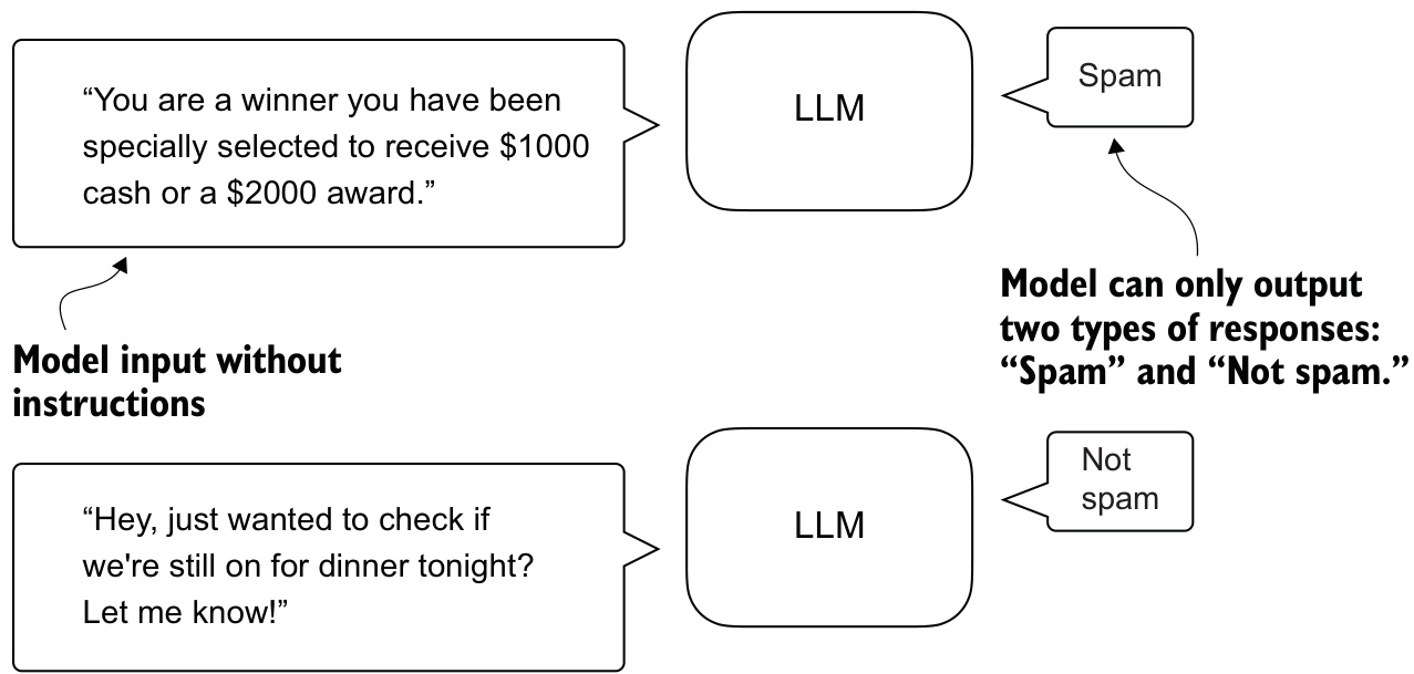
The trade-off is stated in the chapter’s sidebar on choosing the right approach, and it is the whole basis of the decision:
Instruction fine-tuning is best suited to models that must handle a variety of tasks based on complex user instructions, improving flexibility and interaction quality.
It demands larger datasets and greater computational resources to develop models proficient in various tasks.
Classification fine-tuning is ideal for projects requiring precise categorization of data into predefined classes, such as sentiment analysis or spam detection.
It requires less data and compute power, but its use is confined to the specific classes on which the model has been trained.
A classification fine-tuned model is highly specialized, and it is generally easier to develop a specialized model than a generalist model that works well across various tasks.
The distinction is one of output space, not of architecture. Both approaches start from the same pretrained backbone; instruction fine-tuning keeps the vocabulary head so the model can emit arbitrary text, while classification fine-tuning discards it.
Learning outcomes
- choosing-a-fine-tuning-approach Choose between classification and instruction fine-tuning for a given task.
Concepts
- classification-fine-tuning the model is trained to recognize a specific set of class labels, and its output is confined to that set
- instruction-fine-tuning the model is trained on tasks specified as natural language prompts, which yields a generalist at the cost of more data and more compute
Preparing the spam dataset
The worked example uses the SMS Spam Collection, downloaded as a zip archive from the UCI repository and extracted to a tab-separated file:
url = "https://archive.ics.uci.edu/static/public/228/sms+spam+collection.zip"
zip_path = "sms_spam_collection.zip"
extracted_path = "sms_spam_collection"
data_file_path = Path(extracted_path) / "SMSSpamCollection.tsv"
Read into a pandas DataFrame with pd.read_csv(data_file_path, sep="\t", header=None, names=["Label", "Text"]), the dataset has 5,572 rows and two columns. Its label distribution is severely skewed:
Label
ham     4825
spam     747
Name: count, dtype: int64
Dataset undersampling removes the skew by reducing the majority class to the size of the minority class. Raschka’s stated reasons are simplicity and a preference for a small dataset, which facilitates faster fine-tuning of the LLM.
def create_balanced_dataset(df):
    num_spam = df[df["Label"] == "spam"].shape[0]
    ham_subset = df[df["Label"] == "ham"].sample(
        num_spam, random_state=123
    )
    balanced_df = pd.concat([
        ham_subset, df[df["Label"] == "spam"]
    ])
    return balanced_df

balanced_df = create_balanced_dataset(df)
print(balanced_df["Label"].value_counts())
The result is 747 of each class. The string labels are then mapped to integers, because the loss function consumes class indices rather than strings:
balanced_df["Label"] = balanced_df["Label"].map({"ham": 0, "spam": 1})This process is similar to converting text into token IDs. However, instead of using the GPT vocabulary, which consists of more than 50,000 words, we are dealing with just two token IDs: 0 and 1.
The balanced frame is shuffled and cut into three parts — 70% for training, 10% for validation, 20% for testing:
def random_split(df, train_frac, validation_frac):

    df = df.sample(
        frac=1, random_state=123
    ).reset_index(drop=True)
    train_end = int(len(df) * train_frac)
    validation_end = train_end + int(len(df) * validation_frac)

    train_df = df[:train_end]
    validation_df = df[train_end:validation_end]
    test_df = df[validation_end:]

    return train_df, validation_df, test_df

train_df, validation_df, test_df = random_split(
    balanced_df, 0.7, 0.1)
The test fraction is not passed; it is implied to be 0.2 as the remainder. The three frames are written to train.csv, validation.csv and test.csv with index=None, so the splits are fixed and reusable.
Accuracy on an unbalanced set is not interpretable. On the original 4,825/747 split, a model that always answers “ham” scores about 87% while having learned nothing. After undersampling, chance performance is 50%, so every percentage point above it is attributable to the classifier.
Learning outcomes
- preparing-a-balanced-labeled-dataset Download, balance and split a labeled text dataset for supervised fine-tuning.
Concepts
- dataset-undersampling 747 ham messages are drawn at random to match the 747 spam messages, which removes the majority-class bias from the gradient updates
Datasets and data loaders
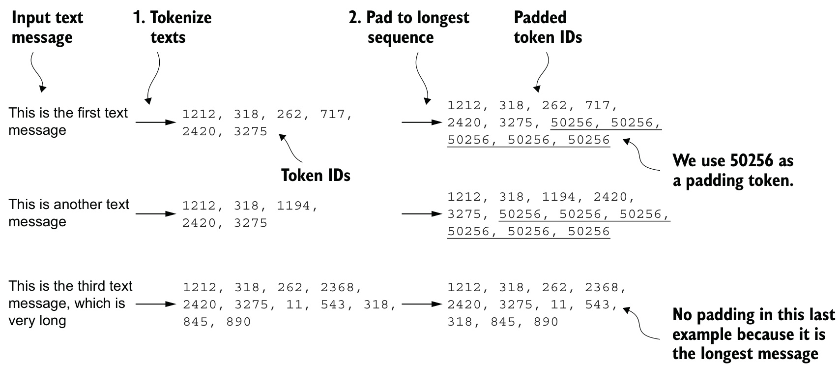
Batching requires every sequence in a batch to be the same length, and text messages are not. The chapter names two options:
- Truncate all messages to the length of the shortest message in the dataset or batch.
- Pad all messages to the length of the longest message in the dataset or batch.
The first option is computationally cheaper, but it may result in significant information loss if shorter messages are much smaller than the average or longest messages, potentially reducing model performance. The second option is chosen, because it preserves the entire content of all messages.
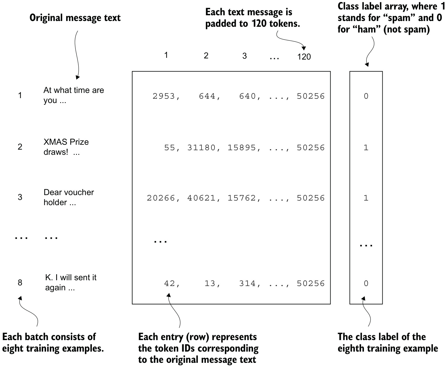
Sequence padding and truncation is implemented with the same GPT-2 tokenizer the pretrained weights expect. The padding token is <|endoftext|>, whose token ID is 50256; tokenizer.encode("<|endoftext|>", allowed_special={"<|endoftext|>"}) returns [50256].
class SpamDataset(Dataset):
    def __init__(self, csv_file, tokenizer, max_length=None,
                 pad_token_id=50256):
        self.data = pd.read_csv(csv_file)

        self.encoded_texts = [
            tokenizer.encode(text) for text in self.data["Text"]
        ]

        if max_length is None:
            self.max_length = self._longest_encoded_length()
        else:
            self.max_length = max_length

            self.encoded_texts = [
                encoded_text[:self.max_length]
                for encoded_text in self.encoded_texts
            ]

        self.encoded_texts = [
            encoded_text + [pad_token_id] *
            (self.max_length - len(encoded_text))
            for encoded_text in self.encoded_texts
        ]

    def __getitem__(self, index):
        encoded = self.encoded_texts[index]
        label = self.data.iloc[index]["Label"]
        return (
            torch.tensor(encoded, dtype=torch.long),
            torch.tensor(label, dtype=torch.long)
        )

    def __len__(self):
        return len(self.data)

    def _longest_encoded_length(self):
        max_length = 0
        for encoded_text in self.encoded_texts:
            encoded_length = len(encoded_text)
            if encoded_length > max_length:
                max_length = encoded_length
        return max_length
Constructed with max_length=None on train.csv, the dataset sets its own max_length from the longest encoded message. print(train_dataset.max_length) outputs 120. The model can handle sequences of up to 1,024 tokens, given its context length limit; for a dataset containing longer texts, max_length=1024 ensures the data does not exceed the model’s supported input length.
The validation and test sets are then built with max_length=train_dataset.max_length. Any validation or test sample exceeding the length of the longest training example is truncated by encoded_text[:self.max_length]. That truncation is optional — max_length=None may be used for both, provided no sequence in those sets exceeds 1,024 tokens.
train_loader = DataLoader(
    dataset=train_dataset,
    batch_size=batch_size,
    shuffle=True,
    num_workers=num_workers,
    drop_last=True,
)
with num_workers = 0, batch_size = 8 and torch.manual_seed(123). The validation and test loaders take the same batch size and drop_last=False. Iterating the training loader and printing the shape of the last batch gives:
Input batch dimensions: torch.Size([8, 120])
Label batch dimensions torch.Size([8])
The label tensor has one entry per example, not one per token. The loaders hold 130 training batches, 19 validation batches and 38 test batches.
Learning outcomes
- padded-datasets-and-loaders Build a PyTorch Dataset that tokenizes and pads variable-length texts to a uniform length.
Concepts
- padding-and-truncation messages are cut at
max_lengthand extended with token ID50256up to it, so every batch is a rectangular tensor of shape \([8, 120]\)
Pretrained weights and frozen layers
The configuration is the one used for pretraining, with the 124M variant selected:
BASE_CONFIG = {
    "vocab_size": 50257,
    "context_length": 1024,
    "drop_rate": 0.0,
    "qkv_bias": True
}
model_configs = {
    "gpt2-small (124M)": {"emb_dim": 768, "n_layers": 12, "n_heads": 12},
    "gpt2-medium (355M)": {"emb_dim": 1024, "n_layers": 24, "n_heads": 16},
    "gpt2-large (774M)": {"emb_dim": 1280, "n_layers": 36, "n_heads": 20},
    "gpt2-xl (1558M)": {"emb_dim": 1600, "n_layers": 48, "n_heads": 25},
}
BASE_CONFIG.update(model_configs[CHOOSE_MODEL])
download_and_load_gpt2 fetches the checkpoint, and GPTModel plus load_weights_into_gpt from the pretraining unit place the tensors:
model_size = CHOOSE_MODEL.split(" ")[-1].lstrip("(").rstrip(")")
settings, params = download_and_load_gpt2(
    model_size=model_size, models_dir="gpt2"
)

model = GPTModel(BASE_CONFIG)
load_weights_into_gpt(model, params)
model.eval()
Generating from the prompt "Every effort moves you" produces Every effort moves you forward. / The first step is to understand the importance of your work, which indicates that the model weights have been loaded correctly. Running this check first separates weight-mapping faults from fine-tuning faults later on.
The same model, prompted with an explicit instruction, does not classify:
Is the following text 'spam'? Answer with 'yes' or 'no': 'You are a winner
you have been specially selected to receive $1000 cash
or a $2000 award.'
The following text 'spam'? Answer with 'yes' or 'no': 'You are a winner
The model is struggling to follow instructions. This result is expected, as it has only undergone pretraining and lacks instruction fine-tuning. The failure is not a shortage of knowledge but a mismatch of objective: next-token prediction continues the prompt, and continuing this prompt means repeating it.
Selective parameter freezing is applied before any training. All parameters are made nontrainable:
for param in model.parameters():
    param.requires_grad = False
Frozen parameters receive no gradients, so the representations acquired during pretraining are unchanged and each optimizer step touches far fewer tensors. Two modules are then returned to the trainable set:
for param in model.trf_blocks[-1].parameters():
    param.requires_grad = True
for param in model.final_norm.parameters():
    param.requires_grad = True
Training the new output layer alone is technically sufficient. Raschka reports that, in his experiments, fine-tuning additional layers can noticeably improve the predictive performance of the model. The reason given for the choice of these two is structural: the lower layers generally capture basic language structures and semantics applicable across a wide range of tasks and datasets, while layers near the output are more specific to nuanced linguistic patterns and task-specific features.
Learning outcomes
- freezing-a-pretrained-backbone Load pretrained GPT-2 weights and freeze the parameters you do not want to train.
Concepts
- parameter-freezing
requires_grad = Falseacross all parameters, thenTrueontrf_blocks[-1]andfinal_norm, leaves the general representations intact while granting the model enough capacity to adapt
The classification head and the last token
print(model) ends with the two modules that matter here:
  (final_norm): LayerNorm()
  (out_head): Linear(in_features=768, out_features=50257, bias=False)
)
A classification head replaces out_head with a linear layer whose output width is the number of classes:
torch.manual_seed(123)
num_classes = 2
model.out_head = torch.nn.Linear(
    in_features=BASE_CONFIG["emb_dim"],
    out_features=num_classes
)
BASE_CONFIG["emb_dim"] is 768 for "gpt2-small (124M)", so writing the width this way lets the same code serve the larger GPT-2 variants. The new layer has its requires_grad attribute set to True by default, which is what makes it the one module guaranteed to be updated during training.
A single output node would suffice for a binary task, but it would require modifying the loss function. Matching the number of output nodes to the number of classes generalizes without change: a three-class problem — classifying news articles as “Technology”, “Sports” or “Politics” — uses three output nodes.
The model still emits one output row per input token. For the four-token input "Do you have time":
Outputs:
 tensor([[[-1.5854,  0.9904],
         [-3.7235,  7.4548],
         [-2.2661,  6.0649],
         [-3.5983,  3.9902]]])
Outputs dimensions: torch.Size([1, 4, 2])
The same input previously produced a tensor of shape [1, 4, 50257]. The number of rows still corresponds to the number of input tokens; only the number of columns has changed.
Last-token prediction pooling selects one of those four rows. The choice follows from the causal attention mask of chapter 3, which restricts a token’s focus to its current position and those before it.
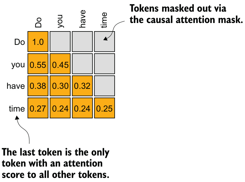
time, is the only one that computes attention scores for all preceding tokens.Given that mask, the last token in a sequence accumulates the most information, since it is the only token with access to all the previous tokens. So the final row is extracted:
print("Last output token:", outputs[:, -1, :])Last output token: tensor([[-3.5983, 3.9902]])The direction of the argument is worth stating precisely: the first token position is unusable here not because it is uninformative in general, but because causal masking denies it any view of what follows. An encoder with bidirectional attention faces no such restriction and pools differently.
Learning outcomes
- replacing-the-output-head Swap the vocabulary projection for a class-sized classification head.
- last-token-classification-logits Take the classification decision from the final token position.
Concepts
- classification-head a
Linear(768, 2)layer stands in for theLinear(768, 50257)vocabulary projection, so the output width equals the number of target classes - last-token-pooling the final position is the only one whose attention scores cover the entire input, so
outputs[:, -1, :]is the representation the class decision is read from
Classification loss and accuracy
A class label is obtained from the last-token logits by the same two operations used for next-token prediction, applied to two-dimensional instead of 50,257-dimensional outputs:
probas = torch.softmax(outputs[:, -1, :], dim=-1)
label = torch.argmax(probas)
print("Class label:", label.item())
Using softmax here is optional, because the largest logit corresponds to the highest probability score. The code simplifies to:
logits = outputs[:, -1, :]
label = torch.argmax(logits)
print("Class label:", label.item())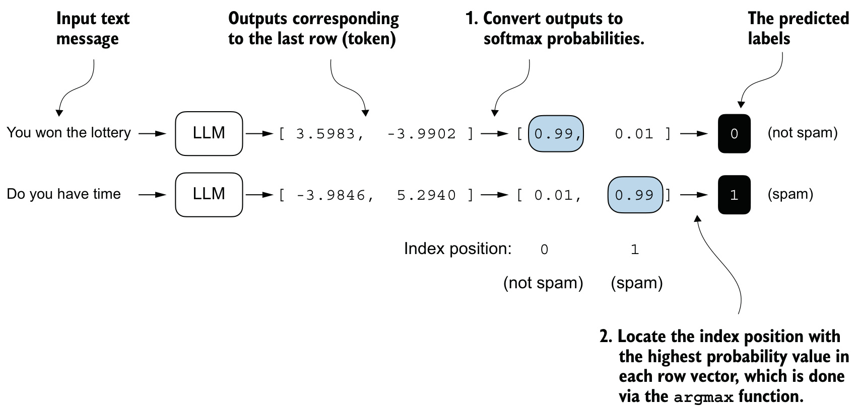
Applied across a loader, this yields the classification accuracy — the percentage of correct predictions across a dataset:
def calc_accuracy_loader(data_loader, model, device, num_batches=None):
    model.eval()
    correct_predictions, num_examples = 0, 0

    if num_batches is None:
        num_batches = len(data_loader)
    else:
        num_batches = min(num_batches, len(data_loader))
    for i, (input_batch, target_batch) in enumerate(data_loader):
        if i < num_batches:
            input_batch = input_batch.to(device)
            target_batch = target_batch.to(device)

            with torch.no_grad():
                logits = model(input_batch)[:, -1, :]
            predicted_labels = torch.argmax(logits, dim=-1)

            num_examples += predicted_labels.shape[0]
            correct_predictions += (
                (predicted_labels == target_batch).sum().item()
            )
        else:
            break
    return correct_predictions / num_examples
Estimated from 10 batches for efficiency, the untrained classifier scores:
Training accuracy: 46.25%
Validation accuracy: 45.00%
Test accuracy: 48.75%
These are near a random prediction, which would be 50% in this case.
Accuracy is what the task cares about, but it is not what the optimizer can use. Because classification accuracy is not a differentiable function, cross-entropy loss is used as a proxy to maximize accuracy. The loss function therefore remains the one from pretraining, with a single adjustment: only the last token is optimized.
def calc_loss_batch(input_batch, target_batch, model, device):
    input_batch = input_batch.to(device)
    target_batch = target_batch.to(device)
    logits = model(input_batch)[:, -1, :]
    loss = torch.nn.functional.cross_entropy(logits, target_batch)
    return loss
calc_loss_loader averages calc_loss_batch over the loader, returning float("nan") when the loader is empty and dividing total_loss by num_batches. Over five batches per split, before training:
Training loss: 2.453
Validation loss: 2.583
Test loss: 2.322Learning outcomes
- classification-loss-and-accuracy Compute classification cross-entropy loss and accuracy over a data loader.
- last-token-classification-logits Take the classification decision from the final token position.
Concepts
- last-token-pooling both
cross_entropyandargmaxare applied tomodel(input_batch)[:, -1, :], so loss and prediction come from the same single position - classification-fine-tuning accuracy is the objective of interest, and differentiable cross-entropy over the label set is the quantity actually minimized
Fine-tuning on supervised data
The training loop is the same overall training loop used for pretraining; the only difference is that the classification accuracy is calculated instead of generating a sample text to evaluate the model. Two further distinctions are named: the number of training examples seen (examples_seen) is tracked instead of the number of tokens, and accuracy is computed after each epoch.
def train_classifier_simple(
        model, train_loader, val_loader, optimizer, device,
        num_epochs, eval_freq, eval_iter):
    train_losses, val_losses, train_accs, val_accs = [], [], [], []
    examples_seen, global_step = 0, -1

    for epoch in range(num_epochs):
        model.train()

        for input_batch, target_batch in train_loader:
            optimizer.zero_grad()
            loss = calc_loss_batch(
                input_batch, target_batch, model, device
            )
            loss.backward()
            optimizer.step()
            examples_seen += input_batch.shape[0]
            global_step += 1

            if global_step % eval_freq == 0:
                train_loss, val_loss = evaluate_model(
                    model, train_loader, val_loader, device, eval_iter)
                train_losses.append(train_loss)
                val_losses.append(val_loss)
                print(f"Ep {epoch+1} (Step {global_step:06d}): "
                      f"Train loss {train_loss:.3f}, "
                      f"Val loss {val_loss:.3f}"
                )

        train_accuracy = calc_accuracy_loader(
            train_loader, model, device, num_batches=eval_iter
        )
        val_accuracy = calc_accuracy_loader(
            val_loader, model, device, num_batches=eval_iter
        )

        print(f"Training accuracy: {train_accuracy*100:.2f}% | ", end="")
        print(f"Validation accuracy: {val_accuracy*100:.2f}%")
        train_accs.append(train_accuracy)
        val_accs.append(val_accuracy)

    return train_losses, val_losses, train_accs, val_accs, examples_seen
evaluate_model is identical to the one used for pretraining. The optimizer and schedule:
torch.manual_seed(123)
optimizer = torch.optim.AdamW(model.parameters(), lr=5e-5, weight_decay=0.1)
num_epochs = 5
with eval_freq=50 and eval_iter=5. The run takes about 6 minutes on an M3 MacBook Air laptop computer and less than half a minute on a V100 or A100 GPU; the reported run completed in 5.65 minutes. Training loss falls from 2.153 at the first logged step to 0.083 at step 000600, and per-epoch accuracy rises 70.00% → 82.50% → 90.00% → 100.00% → 100.00% on training batches, 72.50% → 85.00% → 90.00% → 97.50% → 97.50% on validation batches.
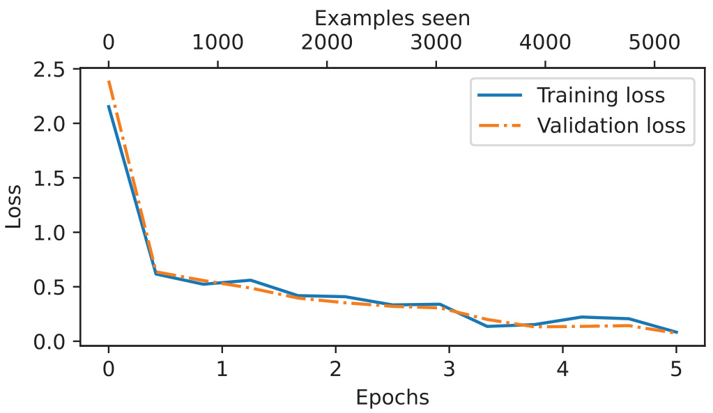
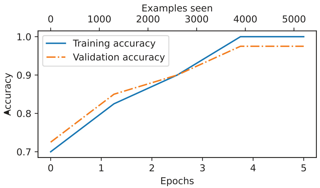
The curves are drawn by plot_values, which places epochs on the primary x-axis and examples seen on a twin axis:
def plot_values(
        epochs_seen, examples_seen, train_values, val_values,
        label="loss"):
    fig, ax1 = plt.subplots(figsize=(5, 3))

    ax1.plot(epochs_seen, train_values, label=f"Training {label}")
    ax1.plot(
        epochs_seen, val_values, linestyle="-.",
        label=f"Validation {label}"
    )
    ax1.set_xlabel("Epochs")
    ax1.set_ylabel(label.capitalize())
    ax1.legend()

    ax2 = ax1.twiny()
    ax2.plot(examples_seen, train_values, alpha=0)
    ax2.set_xlabel("Examples seen")

    fig.tight_layout()
    plt.savefig(f"{label}-plot.pdf")
    plt.show()
The per-epoch figures above are estimates from five batches, since eval_iter=5. Recomputing over the full loaders, without num_batches, gives the final numbers:
Training accuracy: 97.21%
Validation accuracy: 97.32%
Test accuracy: 95.67%
The slight discrepancy between the training and test set accuracies suggests minimal overfitting of the training data. Validation accuracy is somewhat higher than test accuracy because model development often involves tuning hyperparameters to perform well on the validation set, which might not generalize as effectively to the test set — a gap that can be narrowed by raising drop_rate or weight_decay.
The number of epochs depends on the dataset and the task’s difficulty, and there is no universal solution or recommendation, although an epoch number of five is usually a good starting point. If validation loss rises after the first few epochs, reduce the number of epochs; if the trend line suggests the validation loss could improve with further training, increase it.
Learning outcomes
- running-the-supervised-fine-tuning Fine-tune the adapted model with AdamW and read its loss and accuracy curves.
- classification-loss-and-accuracy Compute classification cross-entropy loss and accuracy over a data loader.
Concepts
- classification-fine-tuning five epochs of AdamW at \(5 \times 10^{-5}\) over roughly 1,000 examples move the classifier from chance to 95.67% test accuracy
Using and saving the classifier
Inference on one new string repeats the preprocessing steps of SpamDataset, then predicts an integer class label and returns the corresponding class name:
def classify_review(
        text, model, tokenizer, device, max_length=None,
        pad_token_id=50256):
    model.eval()

    input_ids = tokenizer.encode(text)
    supported_context_length = model.pos_emb.weight.shape[0]

    input_ids = input_ids[:min(
        max_length, supported_context_length
    )]

    input_ids += [pad_token_id] * (max_length - len(input_ids))

    input_tensor = torch.tensor(
        input_ids, device=device
    ).unsqueeze(0)

    with torch.no_grad():
        logits = model(input_tensor)[:, -1, :]
    predicted_label = torch.argmax(logits, dim=-1).item()

    return "spam" if predicted_label == 1 else "not spam"
Three details in that function are the ones a reimplementation gets wrong. The truncation bound is min(max_length, supported_context_length), read from model.pos_emb.weight.shape[0], so a long input cannot exceed the positional embedding table. The padding token is 50256, the same one the dataset used. And max_length is passed as train_dataset.max_length, not chosen afresh — inference must present the model with the shape and padding convention it was trained on.
Two calls, both correct:
text_1 = (
    "You are a winner you have been specially"
    " selected to receive $1000 cash or a $2000 award."
)

print(classify_review(
    text_1, model, tokenizer, device, max_length=train_dataset.max_length
))
returns "spam", and
text_2 = (
    "Hey, just wanted to check if we're still on"
    " for dinner tonight? Let me know!"
)
returns "not spam".
Persistence uses the state_dict mechanism from the pretraining unit:
torch.save(model.state_dict(), "review_classifier.pth")model_state_dict = torch.load("review_classifier.pth", map_location=device)
model.load_state_dict(model_state_dict)Only the parameters are written to disk. Reloading requires an already-constructed model of the same shape — GPTModel(BASE_CONFIG) with out_head replaced by a Linear(768, 2) — otherwise the keys and shapes in the dictionary will not match.
The chapter’s summary states the result in six points, of which four bear on the architecture: classification fine-tuning replaces the output layer of an LLM via a small classification layer; that layer consists of only two output nodes in this task, against 50,256 output nodes for the number of unique tokens in the vocabulary; classification fine-tuning trains the model to output a correct class label rather than to predict the next token in the text; and fine-tuning a classification model uses the same cross entropy loss function as when pretraining the LLM.
Learning outcomes
- deploying-the-classifier Use and persist the fine-tuned classifier on new text.
- padded-datasets-and-loaders Build a PyTorch Dataset that tokenizes and pads variable-length texts to a uniform length.
Concepts
- padding-and-truncation a single inference string is truncated to
min(max_length, supported_context_length)and padded with50256, mirroring the training preprocessing exactly - last-token-pooling
classify_reviewreadslogits[:, -1, :]and maps itsargmaxto"spam"or"not spam" - classification-head the two-node output layer is what the saved
state_dictexpects, so the reloading model must be built with the same replacement - classification-fine-tuning the finished pipeline runs raw text through tokenization, padding, a frozen backbone and a two-class head to a label
- instruction-fine-tuning the alternative adaptation route retains a text-generating head and so answers arbitrary prompts, which this classifier cannot
A specialist built and a generalist ahead
Classification fine-tuning produces a specialist; instruction fine-tuning produces a generalist.
The specialist requires a smaller labeled dataset, fewer epochs and less compute, and its output is confined to the classes it was trained on.
Adapting a causal LLM for classification means replacing the vocabulary projection and freezing most of the backbone.
The \(768 \rightarrow 50257\) head becomes \(768 \rightarrow 2\); the embeddings and the first eleven transformer blocks receive no gradients, so pretrained representations are preserved and the step cost falls.
Causal masking dictates that the classification logits are read from the last token position.
It is the only position whose attention scores cover every preceding token, which is why
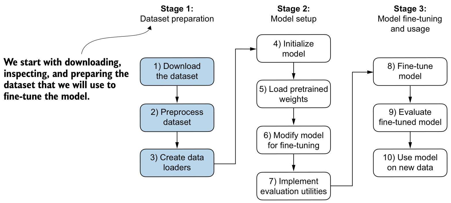
outputs[:, -1, :]and notoutputs[:, 0, :]carries the whole input.The pipeline runs in three stages: dataset preparation, model setup, then fine-tuning, evaluation and use.
Undersampling to 747 per class, padding to 120 tokens with
50256, five epochs of AdamW at \(5 \times 10^{-5}\), and aclassify_reviewcall on a fresh string are the concrete steps, ending at 95.67% test accuracy.Cross-entropy is optimized because accuracy cannot be.
Classification accuracy is not differentiable, so the same loss function used in pretraining serves as its proxy, evaluated at one position instead of all of them.
The next unit, 7 Fine-tuning to follow instructions, takes the other branch of stage 3. The vocabulary head is retained and the training targets become response tokens rather than class indices, which changes the data pipeline: padding is applied per batch to its longest sequence rather than to a dataset-wide max_length, and padded target positions are set to -100 so they contribute no gradient. Capacity becomes a constraint that 124M parameters do not meet, so GPT-2 Medium (355M) is loaded instead. With no fixed label set, accuracy is unavailable as a metric, and the responses are scored instead by a locally hosted Llama 3 model acting as a judge.
References
- Building a Large Language Model (from scratch), Sebastian Raschka, 2024, Manning Books — Link — Page 191-225