6 Fine-tuning for classification

Language Models · v1.0.0

2026-08-25 14:45:44

Where we are

The general-purpose model, finished

In 5 Pretraining on unlabeled data we finished the general-purpose model.

  • Built the LLM architecture.
  • Pretrained it.
  • Imported pretrained weights from OpenAI into our own GPTModel.

The result completes text fluently and knows nothing about any particular task.

Stage 3: fine-tuning

This unit reaps the fruits of that labour — stage 3, step 8: fine-tuning a pretrained LLM as a classifier.

  • Concrete example: classifying text messages as “spam” or “not spam.”
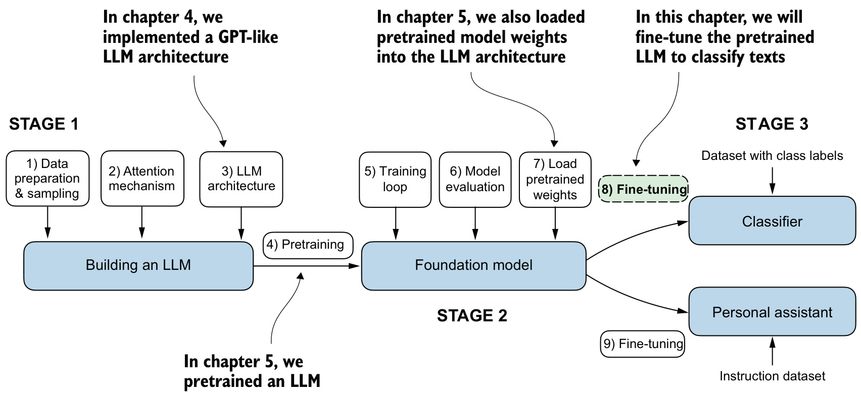
Figure 6.1 The three main stages of coding an LLM. This chapter focuses on stage 3 (step 8): fine-tuning a pretrained LLM as a classifier.

Very little machinery changes

  • We keep the embeddings and eleven of the twelve transformer blocks frozen.
  • We replace the \(768 \rightarrow 50257\) vocabulary projection with a \(768 \rightarrow 2\) head.
  • We read the answer from the last token position, not from every position.
  • The optimizer, the cross-entropy loss, and the loader-averaged evaluation all carry over unchanged.

By the end, a 124M-parameter model fine-tuned on roughly a thousand labeled examples over five epochs classifies unseen messages at 95.67% accuracy.

Which kind of fine-tuning

Two common approaches

The choice is made before any implementation begins — the two differ in the data they need, the compute they cost, and what the finished model can do.

  • Instruction fine-tuning — trains on instructions given in natural language, to execute a variety of tasks.
  • Classification fine-tuning — trains to recognize a specific, fixed set of class labels.
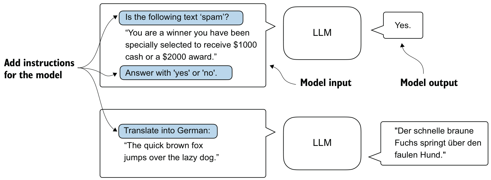
Figure 6.2 Two different instruction fine-tuning scenarios: spam detection, and English-to-German translation.

Classification fine-tuning

The task is not peculiar to language: identifying plant species from images, categorizing news articles, distinguishing benign from malignant tumors.

A classification fine-tuned model is restricted to predicting classes it has encountered during its training.
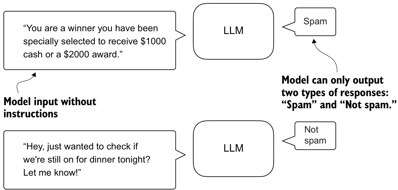
Figure 6.3 A model fine-tuned for spam classification does not require further instruction alongside the input. It can only respond with “spam” or “not spam.”

Choosing the right approach

  • Instruction fine-tuning is best for models handling a variety of tasks based on complex instructions.
  • Classification fine-tuning is ideal for precise categorization into predefined classes.
  • Instruction fine-tuning is more versatile, but demands larger datasets and more compute.
  • Classification fine-tuning needs less data and compute, but is confined to its trained classes.

Preparing the spam dataset

Three stages, this is stage 1

We modify and classification fine-tune the GPT model we previously implemented and pretrained.
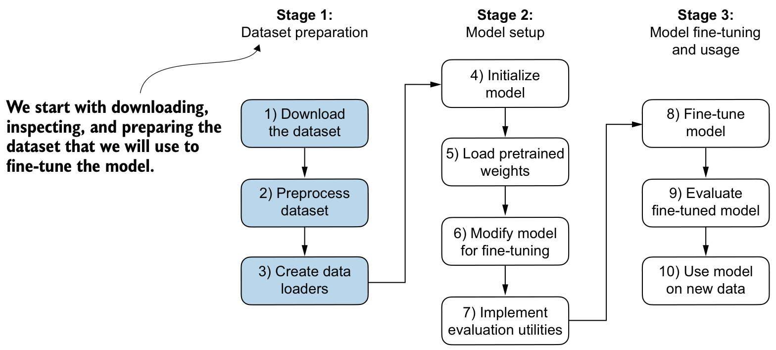
Figure 6.4 The three-stage process for classification fine-tuning an LLM.

  • Dataset: SMS Spam Collection — 5,572 text messages, each tagged ham or spam.

The imbalance, and undersampling

The label counts are far from equal: 4,825 ham against 747 spam. A model that always answered “ham” would be right most of the time and useless.

Dataset undersampling shrinks the majority class to the size of the minority class.

  • Sample 747 ham messages at random; keep all 747 spam.
  • Balanced set of 1,494 — random guessing scores 50%, the baseline to beat.
  • Labels mapped to integers: ham \(\to 0\), spam \(\to 1\).

The split

The balanced set is shuffled and split 70/10/20 into training, validation and test.

  • Ratios common enough in machine learning practice to be a reasonable default.
  • Each split is persisted so the rest of the pipeline can be re-run without repeating the preparation.

Datasets and data loaders

Uniform length, unlike before

The sliding window from the text-data unit does not apply here — messages have varying lengths, and a batch must be a rectangular tensor.

  • Truncate to the shortest message: cheap, but loses information.
  • Pad to the longest message: preserves content — the option we take.

Sequence padding and truncation: we append the token ID 50256 ("<|endoftext|>"), from the same GPT-2 tokenizer.
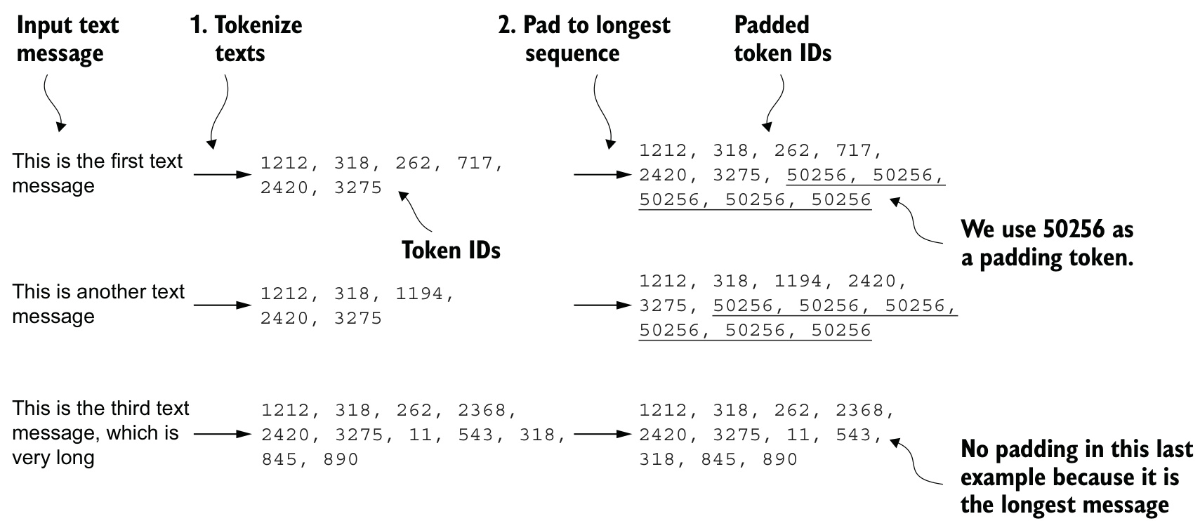
Figure 6.6 Shorter sequences are padded with token ID 50256 to match the length of the longest sequence.

Building the dataset

Conceptually: encode every message, find the longest encoded sequence in the training split, and pad (or truncate) every sequence to that common length.

# pseudo-code
class SpamDataset:
    def build(rows, tokenizer, max_length=None):
        encoded = [tokenizer.encode(text) for text in rows.text]
        max_length = max_length or max(len(e) for e in encoded)
        encoded = [pad_or_truncate(e, max_length, pad_id=EOT_ID) for e in encoded]
        return encoded, rows.label

max_length=None on the training set discovers 120 tokens as typical — well inside GPT-2’s 1,024-token context limit.

The loaders

Standard PyTorch data loaders wrap the dataset.

  • Training loader shuffles and drops a trailing partial batch.
  • Validation and test loaders do neither.
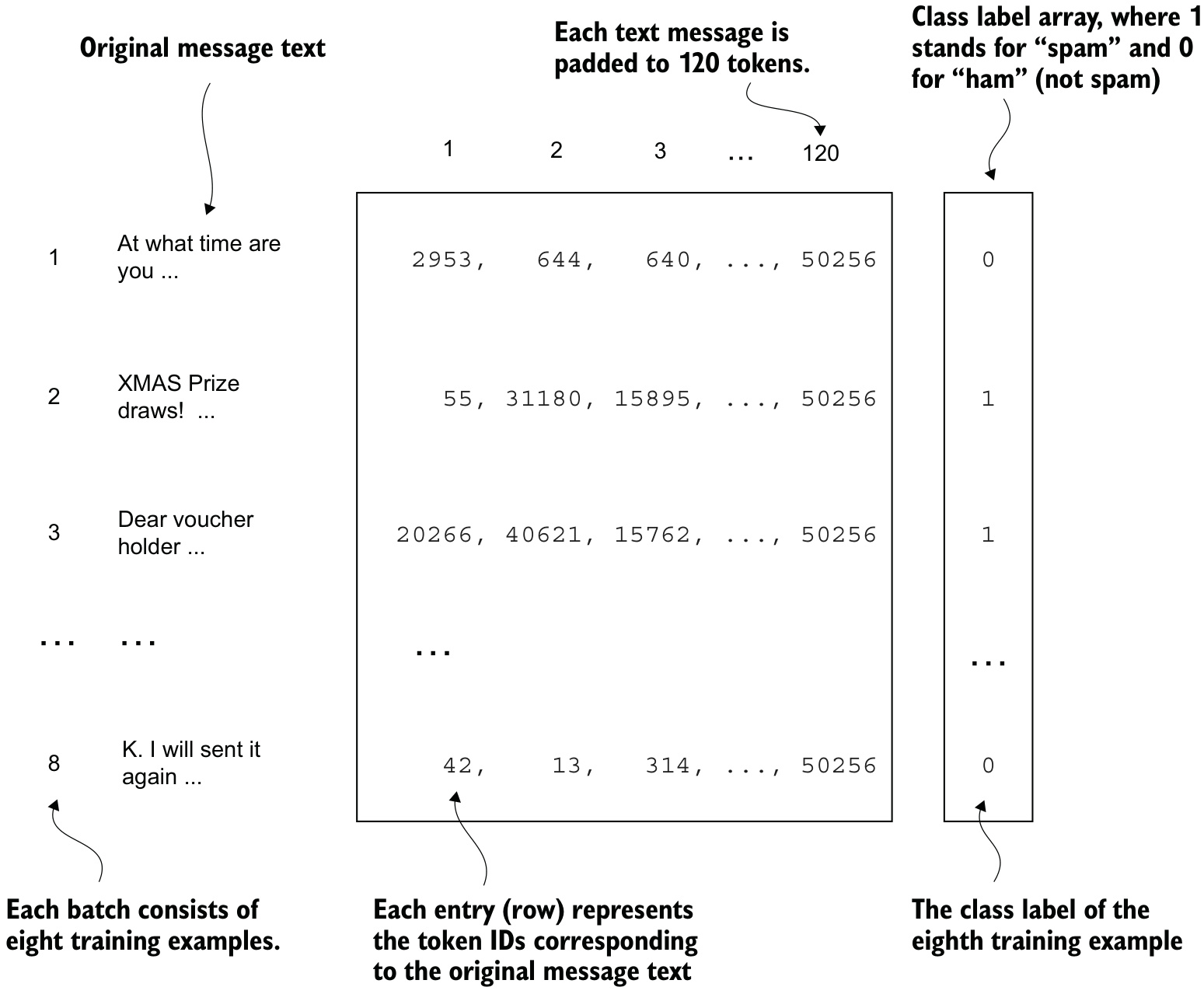
  • Batch size 8 → a (8, 120) tensor of token IDs, paired with an (8,) tensor of labels.

Figure 6.7 A single training batch: eight messages as token IDs, with a class label array.

What makes this classification

The targets are class labels, not the next tokens in the text.

  • One integer per example, not one target per position.
  • The splits hold 130 training batches, 19 validation batches, 38 test batches.

Pretrained weights and frozen layers

Stage 2 begins

We reuse the same GPT-2 configuration and weight-loading utilities from pretraining to obtain a GPTModel populated with pretrained parameters, in evaluation mode.

Two sanity checks

  • Check 1: continuing “Every effort moves you” produces coherent, grammatical text — confirms the weights loaded.
  • Check 2: prompted directly — “Is the following text ‘spam’? Answer with ‘yes’ or ‘no’: …” — the pretrained model simply repeats and continues the prompt.

It struggles to follow instructions, as expected of a model that has only undergone pretraining. Fine-tuning is necessary.

Freezing

Lower layers generally capture basic language structures applicable across many tasks; upper layers are more task-specific.

Selective parameter freezing disables gradients on every parameter as a starting point:

for p in model.parameters():
    p.requires_grad = False

A small part of the model is re-enabled once the new head is in place.

The trade-off

Fewer trainable parameters means faster training and less overfitting risk on ~1,000 examples. Too few, and the model cannot adapt at all.

The classification head and the last token

The head

We replace the \(768 \rightarrow 50257\) output layer with a smaller classification head: \(768 \rightarrow 2\).
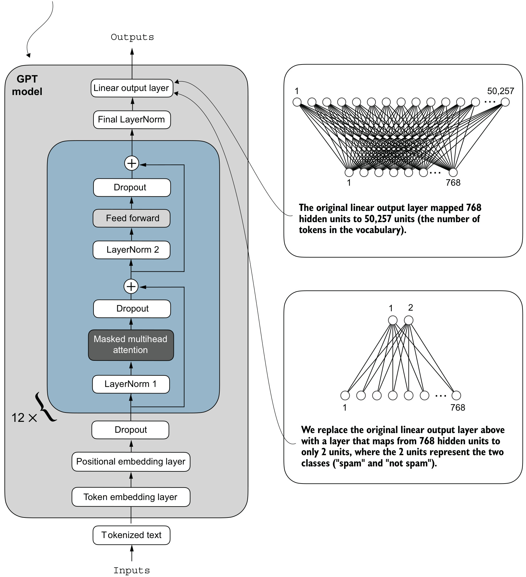
Figure 6.9 Replacing the vocabulary projection with a two-class output layer.

Which layers train

Training the head alone is sufficient, but fine-tuning additional layers noticeably improves performance — so the last transformer block and final LayerNorm are also made trainable.
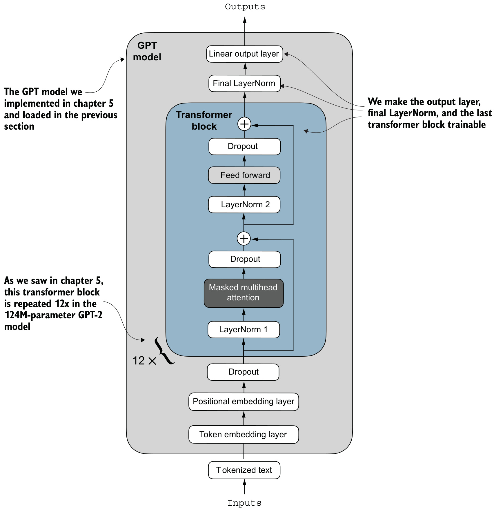
Figure 6.10 The final LayerNorm and the last transformer block are trainable; the remaining 11 blocks and embeddings stay frozen.

The position

A four-token input produces a \(4 \times 2\) tensor of logits, not \(4 \times 50257\). We need one prediction per example, so we keep only the last position: \(\text{logits}[:, -1, :]\).
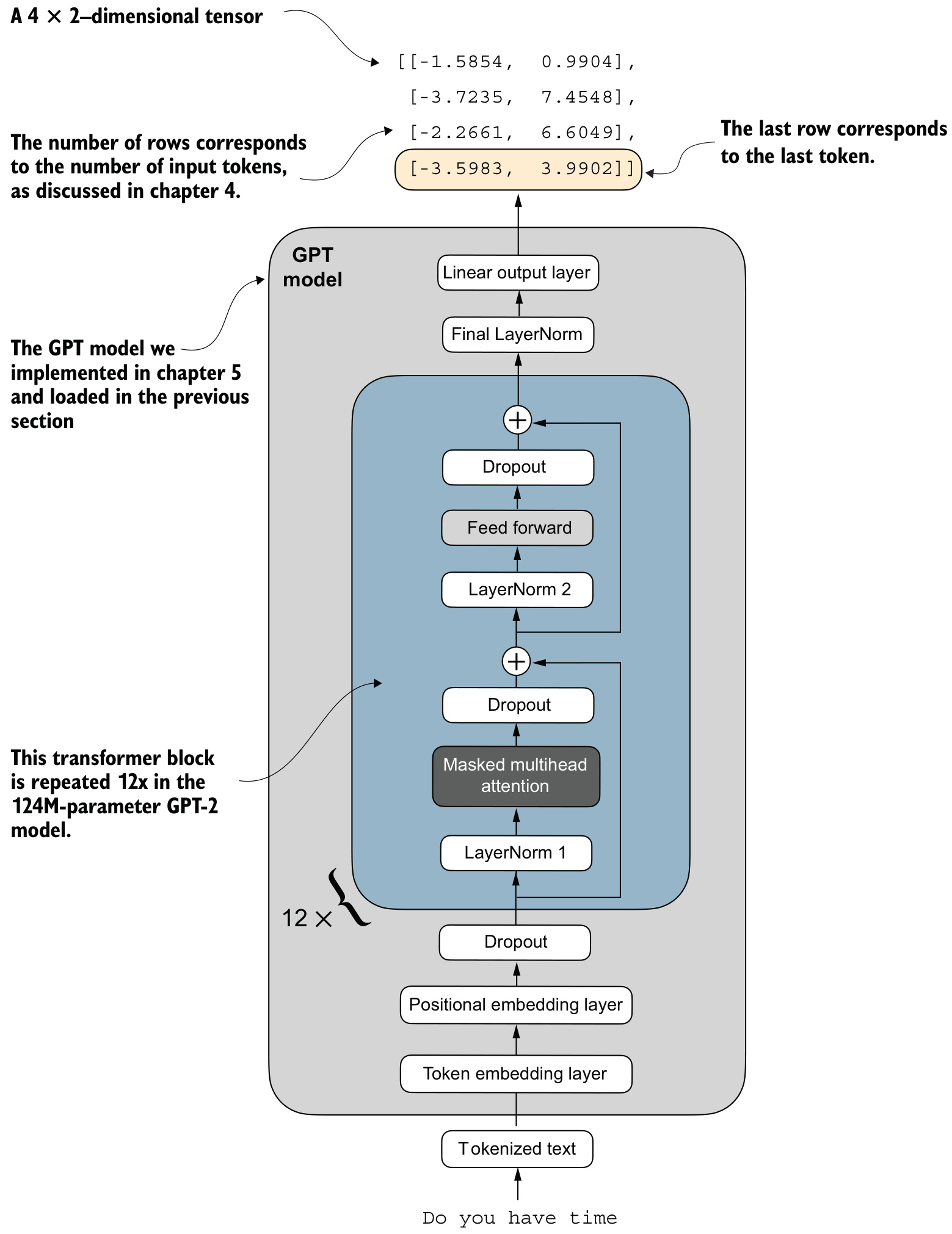
Figure 6.11 Only the last row of the output tensor is used for classification.

Why the last position

Because of the causal attention mask: a token’s focus is restricted to itself and the positions before it.

The last token accumulates the most information since it is the only one with access to all previous tokens.
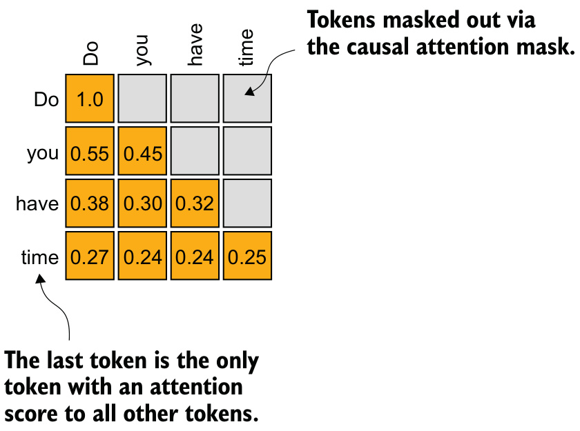
Figure 6.12 The last token, “time”, is the only one that computes attention scores for all preceding tokens.

Classification loss and accuracy

From logits to a label

The two class logits are converted to a label by taking the position of the highest value. Softmax is unnecessary — it does not change which position is largest:

\[ \hat{y} = \arg\max_c \; \text{logits}[-1, c] \]
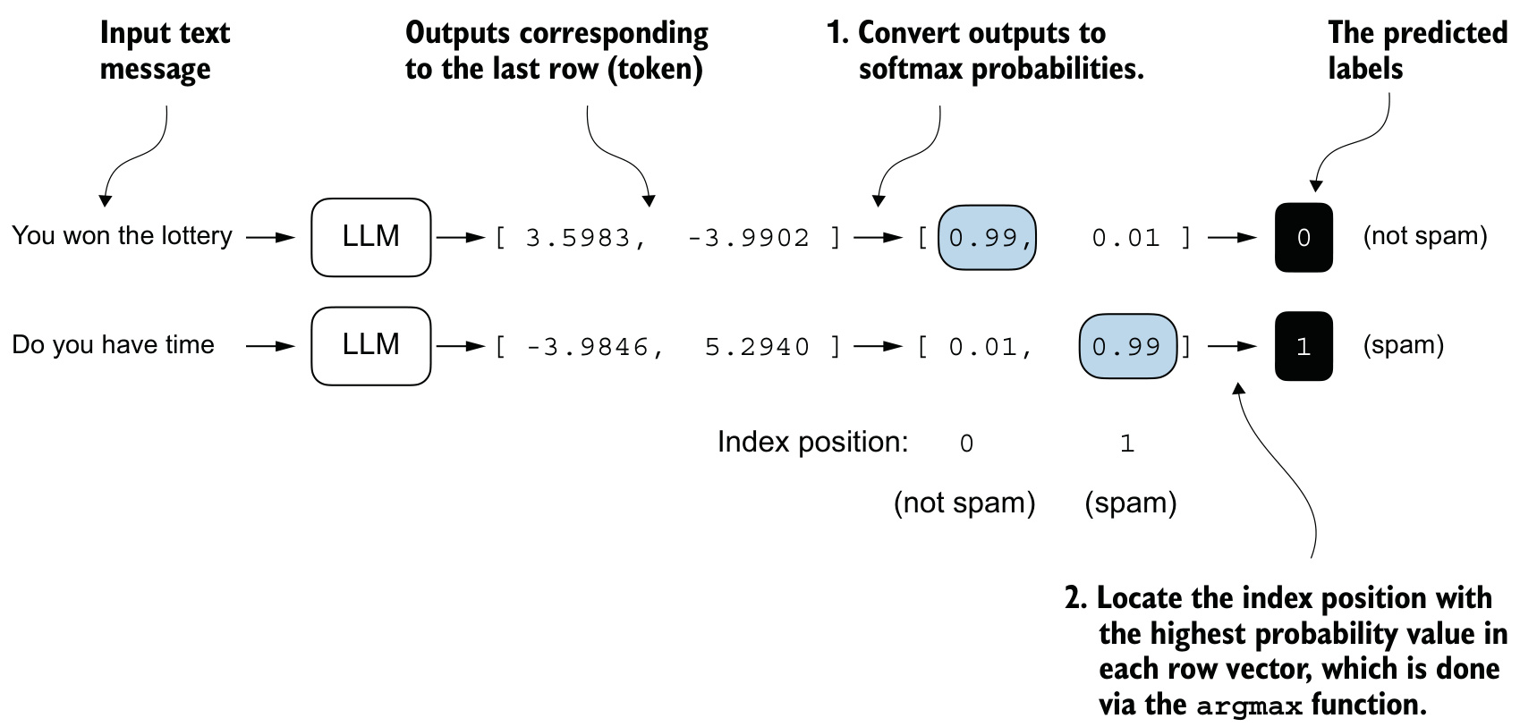
Figure 6.14 Class labels obtained by looking up the highest-probability index. The model predicts incorrectly because it has not yet been trained.

Accuracy over a loader

Classification accuracy: the fraction of examples whose predicted label matches the target label.

Before any fine-tuning, evaluated over ten batches:

  • 46.25% training, 45.00% validation, 48.75% test.
  • Near the 50% random-guess floor, as expected of a randomly initialized head.

The loss

Cross-entropy loss is the differentiable proxy we optimize, applied only to the last-position logits:

\[ \mathcal{L} = \text{CrossEntropy}\big(\text{logits}[:, -1, :],\; y\big) \]

Before fine-tuning: 2.453 training, 2.583 validation, 2.322 test.

Key ideas

  • Cross-entropy is what we optimize; accuracy is what we care about. They are not the same function.
  • On a balanced dataset the accuracy figure is directly interpretable, and 50% is the floor.
  • Both metrics read from the last token position. That single restriction is the entire adaptation of the pretraining evaluation code.

Fine-tuning on supervised data

Same loop, one difference

The training loop is the same overall loop used for pretraining. After each epoch we compute classification accuracy instead of generating a sample text.
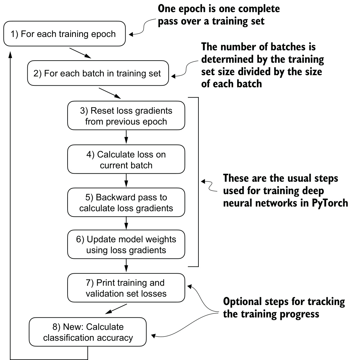
Figure 6.15 A typical training loop: iterate over batches, compute loss, derive gradients, update weights.

The loop

# pseudo-code
def fine_tune(model, train_loader, val_loader, optimizer, num_epochs):
    for epoch in range(num_epochs):
        for inputs, targets in train_loader:
            loss = cross_entropy(model(inputs)[:, -1, :], targets)
            loss.backward(); optimizer.step(); optimizer.zero_grad()
            periodically: log(loss on train_loader, val_loader)
        log(accuracy on train_loader, val_loader)

The optimizer is handed every model parameter; the frozen ones simply receive no gradient.

Running it

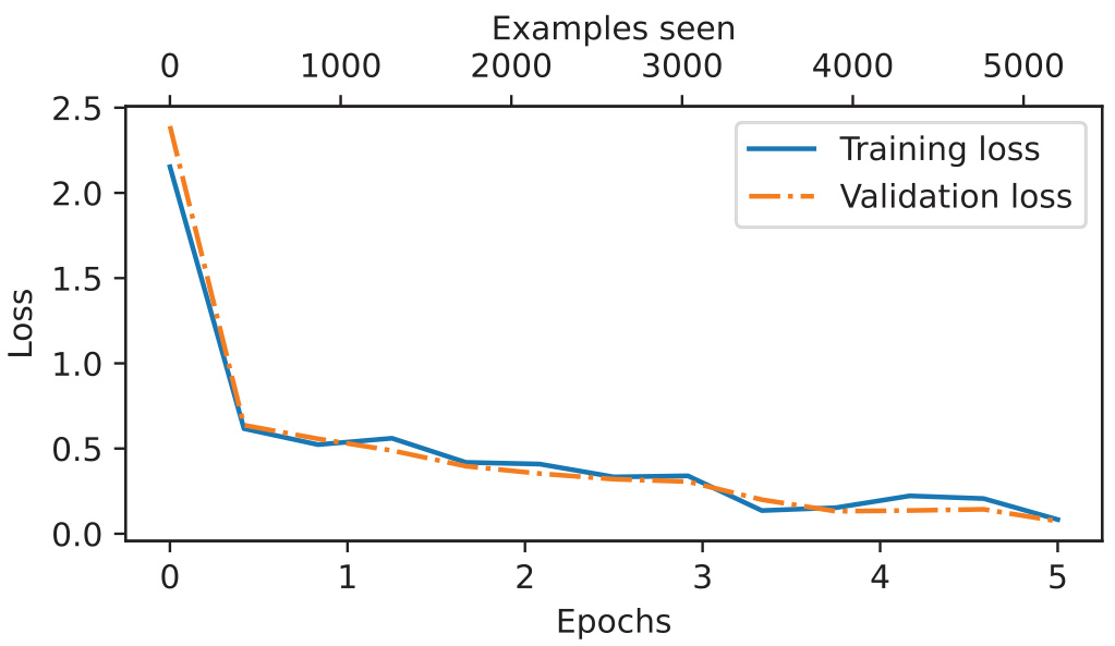
AdamW, learning rate \(5\times 10^{-5}\), weight decay \(0.1\), five epochs.

  • About six minutes on a laptop CPU, under half a minute on a datacenter GPU.
  • Epoch 1: training loss 2.153, 70.00% accuracy.
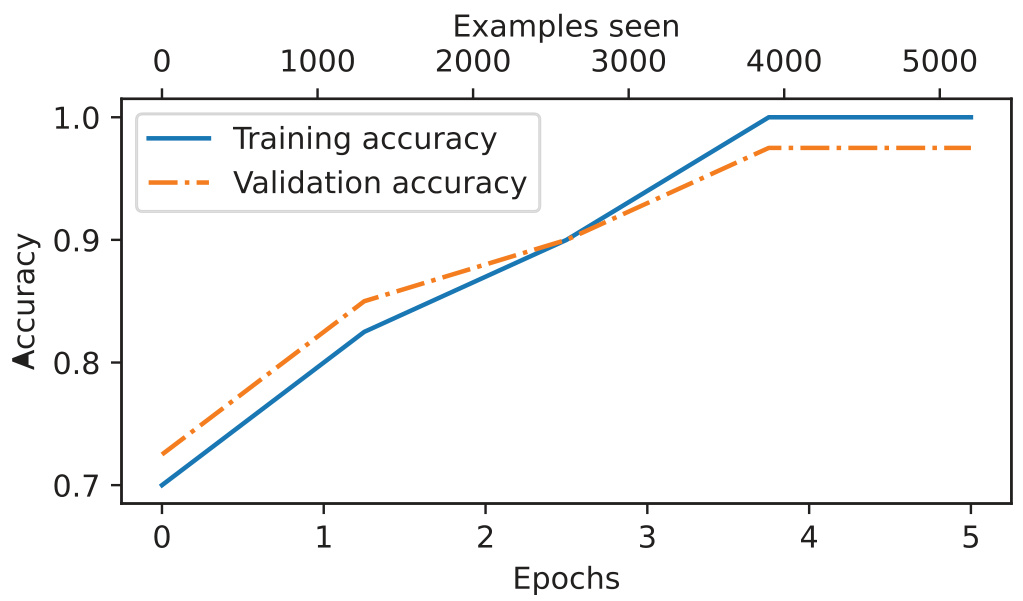
  • Epoch 5: 100.00% training, 97.50% validation accuracy.

The curves

Figure 6.16 Training and validation loss over five epochs.

Figure 6.17 Training and validation accuracy over five epochs.

Little to no indication of overfitting — no noticeable gap between training and validation losses.

Final numbers

Recomputed over the full loaders:

  • 97.21% training
  • 97.32% validation
  • 95.67% test

The slight discrepancy between training and test accuracy suggests minimal overfitting. Validation accuracy is typically somewhat higher than test, because model development tunes hyperparameters against the validation set.

Using and saving the classifier

Step 10, the final step

Having fine-tuned and evaluated the model, we are ready to classify new messages.
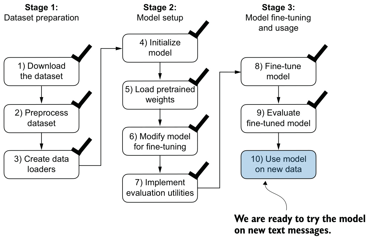
Figure 6.18 Step 10 — using the fine-tuned model to classify new spam messages.

Classifying a new message

Inference repeats exactly the preprocessing done at training time: tokenize, truncate to the shorter of max_length and the model’s context length, pad back to max_length, add a batch dimension.

# pseudo-code
def classify(text, model, tokenizer, max_length):
    ids = tokenizer.encode(text)
    ids = pad_or_truncate(ids, max_length, pad_id=EOT_ID)
    logits = model(as_batch(ids))[:, -1, :]
    return "spam" if argmax(logits) == 1 else "not spam"

Inference must mirror training. A mismatch here does not raise an error; it silently degrades accuracy.

Two examples

  • “You are a winner you have been specially selected to receive $1000 cash or a $2000 award” → correctly predicted spam.
  • “Hey, just wanted to check if we’re still on for dinner tonight? Let me know!” → correctly predicted not spam.

Persistence

Only the weights are saved, never the architecture.

  • Reloading requires constructing a model with the same configuration and the same replaced classification head.
  • Load the saved state into it — otherwise the saved parameters will not match the model’s structure.

What to carry away

Summary \(^1/_2\)

  • Different strategies exist for fine-tuning LLMs: classification and instruction fine-tuning.
  • Classification fine-tuning replaces the output layer with a small classification layer.
  • Instead of predicting the next token as in pretraining, classification fine-tuning trains the model to output a correct class label — only the target changes.

Summary \(^2/_2\)

  • The last token is the position we read, because causal masking gives it access to every preceding token — a property of the architecture, not a convenience.
  • Before fine-tuning, we load the pretrained model as a base model, freezing all but the last transformer block, the final LayerNorm, and the new head.
  • Fine-tuning uses the same cross-entropy loss as pretraining; evaluation adds classification accuracy, since accuracy is not differentiable.

One thing, done well

The model we have built does exactly one thing.

  • Ask it anything other than “is this spam?” and it has no answer.
  • The vocabulary head that could have produced words is gone.

Where next

Next: 7 Fine-tuning to follow instructions.

  • Keeps the language modeling head; trains on prompt-response pairs instead of labels.
  • Produces the generalist this unit deliberately declined to build.

The dataset preparation, freezing, and training-loop patterns reappear; what changes is the target and how success is measured.