Lecture notes — 7 Fine-tuning to follow instructions
ver. 1.2.0, 7_fine_tuning_to_follow_instructions
← 7 Fine-tuning to follow instructions
ver. 1.2.0 · 2026-09-02 16:27:50
Where this fits
The previous unit, 6 Fine-tuning for classification, replaced GPT-2’s vocabulary projection — a Linear(768, 50257) — with a two-unit classification head, froze the lower layers, and read the class logits from the final token position. The result was a spam classifier with a fixed label set of two.
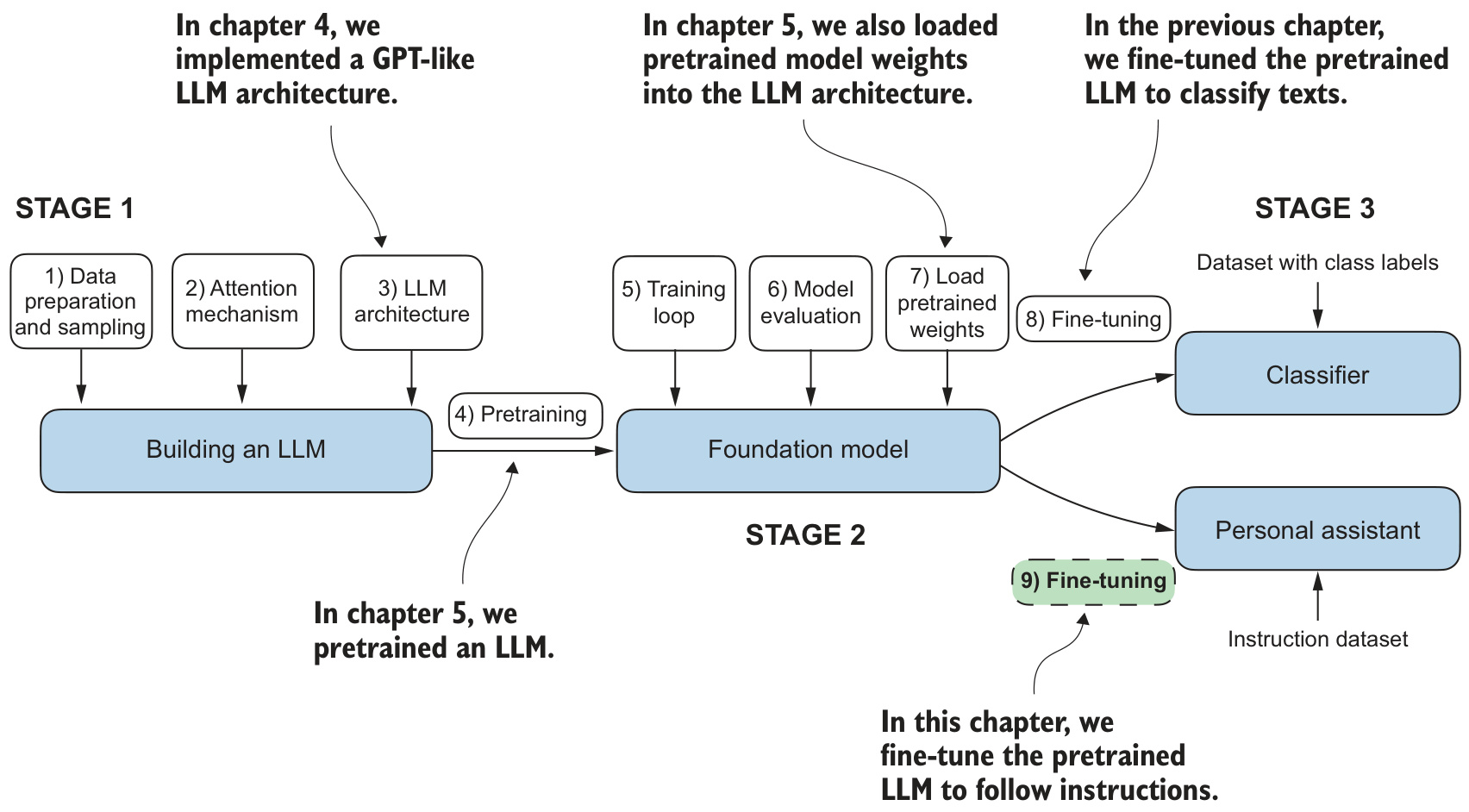
Instruction fine-tuning keeps the language modeling head and changes the targets from class indices to full text responses. The loss remains next-token cross entropy; what changes is the data distribution the model is trained on and the way padding is handled inside it. Figure 7.1 of Building a Large Language Model (from scratch) places both procedures in stage 3 of building an LLM: step 8 produces a classifier, step 9 produces a personal assistant.
Four things are new relative to the classification pipeline: a prompt template that marks where a response begins, per-batch dynamic padding with a -100 loss mask, a larger checkpoint (GPT-2 medium, 355 million parameters), and an evaluation procedure that does not reduce to accuracy.
Learning outcomes
instruction-tuning-versus-base-pretraining— Explain why a pretrained base LLM cannot follow instructions and what instruction fine-tuning changes.alpaca-style-prompt-formatting— Format instruction records into a consistent prompt template.instruction-dataset-and-splits— Load an instruction dataset, split it, and wrap it in a PyTorch Dataset.dynamic-padding-collate-function— Write a custom collate function that pads each batch to its own longest sequence.loss-masking-with-ignore-index— Mask padding targets so they contribute nothing to the gradient.choosing-model-capacity— Justify the choice of GPT-2 Medium over GPT-2 Small for instruction following.running-instruction-fine-tuning— Fine-tune the model on instruction data and interpret the loss curves.extracting-and-saving-responses— Generate responses over a test set and persist them for evaluation.llm-as-a-judge-evaluation— Score open-ended responses automatically with a local LLM judge.next-steps-beyond-this-module— Name the techniques and tools that extend fine-tuning beyond what we built.
Concepts introduced
- Instruction fine-tuning — supervised training of a pretrained base model on instruction–response pairs, so that it answers a request rather than continuing it. Also called supervised instruction fine-tuning.
- Prompt templates — fixed textual schemas that separate the instruction, an optional context input, and the target response within one string. The Alpaca and Phi-3 styles are the two examined here.
- Custom batch collate function — the function a PyTorch
DataLoadercalls to merge a list of samples into batch tensors. Written by hand here to pad per batch, build shifted targets, apply the loss mask, and transfer tensors to the device. - Target loss masking with
ignore_index— replacing target token IDs with-100, the defaultignore_indexof PyTorch’s cross entropy, so those positions are excluded from the loss average. - LLM-as-a-judge — scoring generated responses by presenting the instruction, the reference output and the response to a second, more capable model and reading back a numeric score.
- Ollama — an open source application wrapping the
llama.cpplibrary, which runs LLM inference locally and exposes a REST API athttp://localhost:11434.
Why base models do not follow instructions
Pretraining optimizes one objective: predict the next token. The resulting model is capable of text completion, meaning it can finish sentences or write paragraphs given a fragment as input. Nothing in that objective rewards obeying a request. Pretrained LLMs consequently struggle with specific instructions such as “Fix the grammar in this text” or “Convert this text into passive voice.”
Instruction fine-tuning, also known as supervised instruction fine-tuning, corrects this by further training the pretrained model on explicit input–output pairs. Each pair states a task and the response that task should produce, as in figure 7.2: the instruction “Convert 45 kilometers to meters” is paired with the desired response “45 kilometers is 45000 meters.”
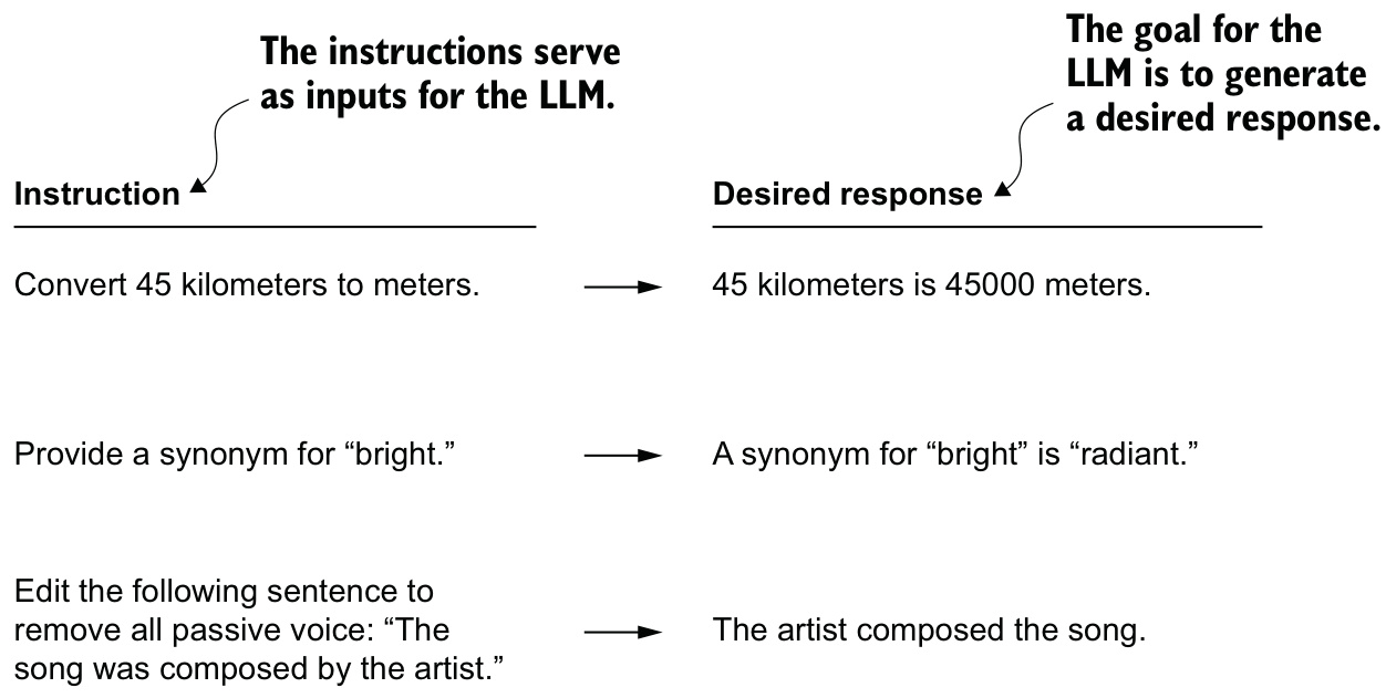
The procedure divides into three stages, shown in figure 7.3.
Stage 1 — preparing the dataset. Dataset download and formatting, batching the dataset, creating data loaders.
All three steps concern data. The training loop itself is reused unchanged from pretraining.
Stage 2 — fine-tuning the LLM. Loading a pretrained LLM, instruction fine-tuning the LLM, inspecting the modeling loss.
Stage 3 — evaluating the LLM. Extracting responses, qualitative evaluation, scoring the responses.
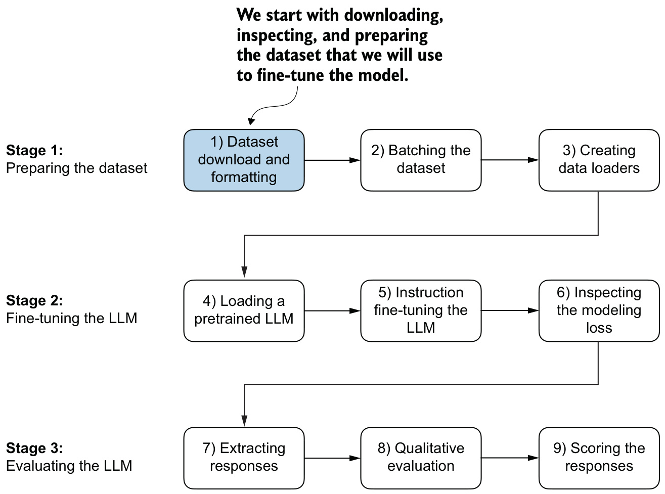
Figure 7.1 of the chapter places this work as step 9 of stage 3 in the larger arc of coding an LLM. Step 8, fine-tuning for classification, was the previous unit; both start from the same foundation model.
Learning outcomes
- instruction-tuning-versus-base-pretraining Explain why a pretrained base LLM cannot follow instructions and what instruction fine-tuning changes.
Concepts
- instruction-fine-tuning supervised training on instruction–response pairs, applied to a model whose pretraining objective rewards continuation rather than obedience
Formatting the instruction dataset
The dataset consists of 1,100 instruction–response pairs, distributed as a 204 KB JSON file. Each entry is a Python dictionary with three keys. Entry 50 is
Example entry:
 {'instruction': 'Identify the correct spelling of the following word.',
  'input': 'Ocassion', 'output': "The correct spelling is 'Occasion.'"}
and entry 999 shows that the 'input' field may occasionally be empty:
Another example entry:
 {'instruction': "What is an antonym of 'complicated'?",
  'input': '',
  'output': "An antonym of 'complicated' is 'simple'."}
The Alpaca prompt style
Figure 7.4 compares two prompt templates. The Alpaca style uses a preamble followed by the headers ### Instruction:, ### Input: and ### Response:. The Phi-3 style is shorter, delimiting turns with the tokens <|user|> and <|assistant|>. Alpaca was among the earliest LLMs to publicly detail its instruction fine-tuning process, and the chapter uses that style throughout.
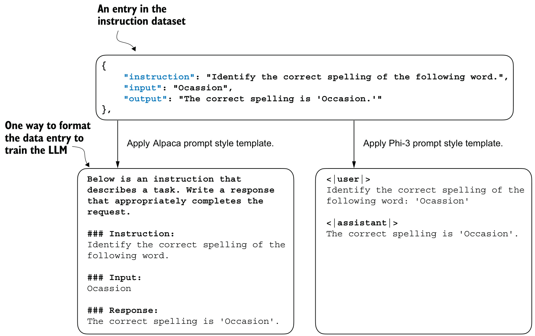
Listing 7.2 renders an entry into the Alpaca format:
def format_input(entry):
    instruction_text = (
        f"Below is an instruction that describes a task. "
        f"Write a response that appropriately completes the request."
        f"\n\n### Instruction:\n{entry['instruction']}"
    )

    input_text = (
        f"\n\n### Input:\n{entry['input']}" if entry["input"] else ""
    )
    return instruction_text + input_text
format_input returns the prompt only. The target text is appended separately as f"\n\n### Response:\n{data[50]['output']}", which for entry 50 yields
Below is an instruction that describes a task. Write a response that
appropriately completes the request.

### Instruction:
Identify the correct spelling of the following word.

### Input:
Ocassion

### Response:
The correct spelling is 'Occasion.'
The conditional expression in input_text is what makes the ### Input: section optional: applied to entry 999, whose 'input' field is the empty string, the formatted prompt contains no ### Input: block at all. The ### Response: marker is the boundary the model learns to treat as its cue to begin answering, and it is the string used later to strip the prompt back off a generated continuation.
Partitioning
Listing 7.3 computes the portions from the length of data:
train_portion = int(len(data) * 0.85)
test_portion = int(len(data) * 0.1)
val_portion = len(data) - train_portion - test_portion

train_data = data[:train_portion]
test_data = data[train_portion:train_portion + test_portion]
val_data = data[train_portion + test_portion:]
The validation portion is the remainder rather than a third percentage, so the three subsets exhaust the 1,100 entries exactly. The printed sizes are 935 training, 55 validation and 110 test examples.
Learning outcomes
- alpaca-style-prompt-formatting Format instruction records into a consistent prompt template.
- instruction-dataset-and-splits Load an instruction dataset, split it, and wrap it in a PyTorch Dataset.
Concepts
- prompt-templates a fixed schema of preamble,
### Instruction:, optional### Input:and### Response:renders every record the same way, which is what makes the response boundary learnable
Batching with a custom collate function
Figure 7.6 breaks the batching process into five substeps: (2.1) apply the prompt template, (2.2) tokenize, (2.3) add padding tokens, (2.4) create target token IDs, and (2.5) replace padding tokens in the targets with placeholders.
Pre-tokenizing the dataset
Steps 2.1 and 2.2 happen once, in the constructor of InstructionDataset (listing 7.4):
import torch
from torch.utils.data import Dataset

class InstructionDataset(Dataset):
    def __init__(self, data, tokenizer):
        self.data = data
        self.encoded_texts = []
        for entry in data:
            instruction_plus_input = format_input(entry)
            response_text = f"\n\n### Response:\n{entry['output']}"
            full_text = instruction_plus_input + response_text
            self.encoded_texts.append(
                tokenizer.encode(full_text)
            )

    def __getitem__(self, index):
        return self.encoded_texts[index]

    def __len__(self):
        return len(self.data)
The prompt and its response are concatenated into full_text and encoded together, so a sample is a single flat list of token IDs. The tokenizer is called once per entry rather than once per entry per epoch.
Dynamic padding
The padding token is <|endoftext|>. Its ID is obtained from the tokenizer rather than assumed:
import tiktoken
tokenizer = tiktoken.get_encoding("gpt2")
print(tokenizer.encode("<|endoftext|>", allowed_special={"<|endoftext|>"}))
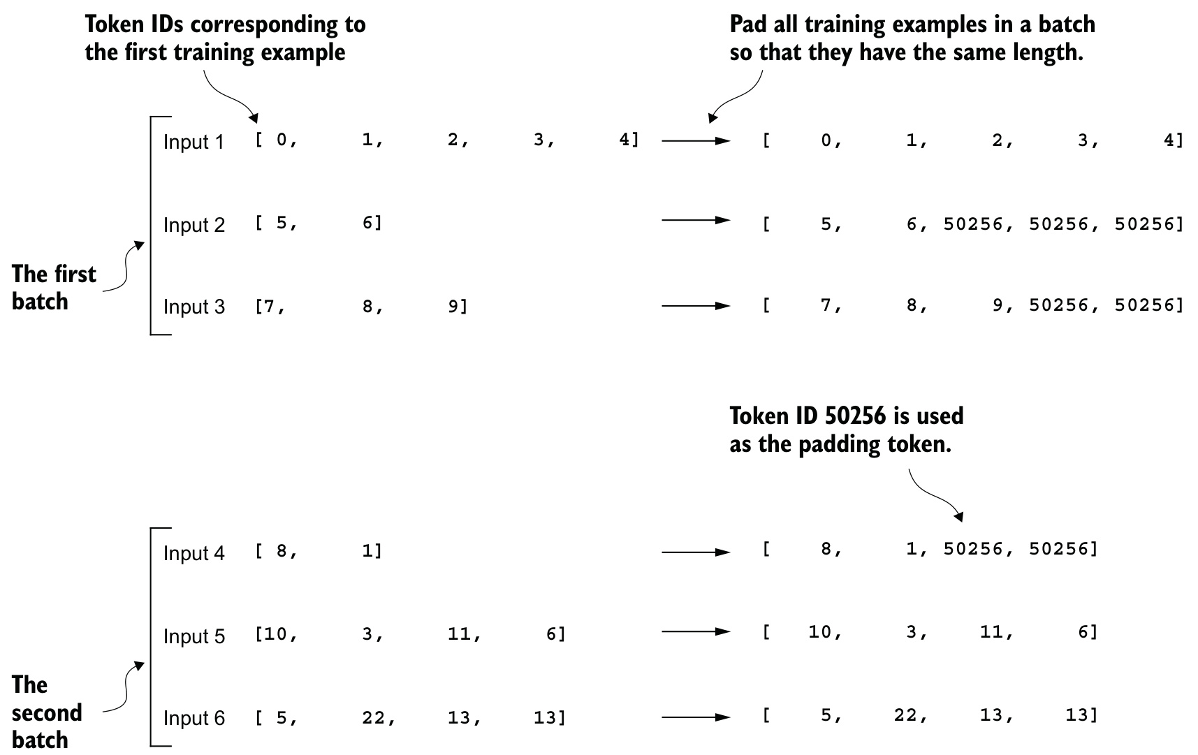
The resulting token ID is 50256. Figure 7.8 shows the padding rule: examples are extended to the length of the longest example in their own batch, so the first batch and the second batch may have different widths. This minimizes unnecessary padding by only extending sequences to match the longest one in each batch, not the whole dataset.
Targets are inputs shifted by one
Figure 7.10 gives the input–target alignment. The target sequence omits the first input token and has an end-of-text token appended, so position \(i\) of the target is the token the model must predict at position \(i\) of the input.
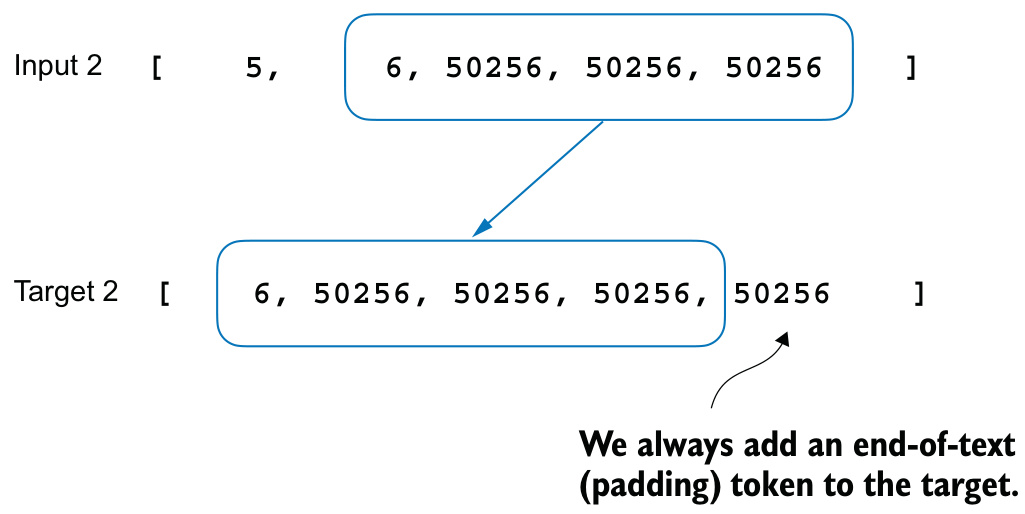
Both tensors come from one padded list, sliced two ways: inputs = torch.tensor(padded[:-1]) and targets = torch.tensor(padded[1:]). That is why batch_max_length is computed as max(len(item)+1 for item in batch) — one extra position is padded on so that both slices are batch_max_length - 1 long.
Masking the padding
Listing 7.5 is the finished collate function:
def custom_collate_fn(
    batch,
    pad_token_id=50256,
    ignore_index=-100,
    allowed_max_length=None,
    device="cpu"
):
    batch_max_length = max(len(item)+1 for item in batch)
    inputs_lst, targets_lst = [], []

    for item in batch:
        new_item = item.copy()
        new_item += [pad_token_id]

        padded = (
            new_item + [pad_token_id] *
            (batch_max_length - len(new_item))
        )
        inputs = torch.tensor(padded[:-1])
        targets = torch.tensor(padded[1:])

        mask = targets == pad_token_id
        indices = torch.nonzero(mask).squeeze()
        if indices.numel() > 1:
            targets[indices[1:]] = ignore_index

        if allowed_max_length is not None:
            inputs = inputs[:allowed_max_length]
            targets = targets[:allowed_max_length]

        inputs_lst.append(inputs)
        targets_lst.append(targets)

    inputs_tensor = torch.stack(inputs_lst).to(device)
    targets_tensor = torch.stack(targets_lst).to(device)
    return inputs_tensor, targets_tensor
The slice indices[1:] is the step most easily misread. indices holds every position where the target equals 50256; dropping the first one means the earliest end-of-text token in each target is left unmasked, and only the later ones become -100. Retaining it allows the LLM to learn when to generate an end-of-text token, which serves as the indicator that a response is complete. Figure 7.12 shows the rule applied to three targets.
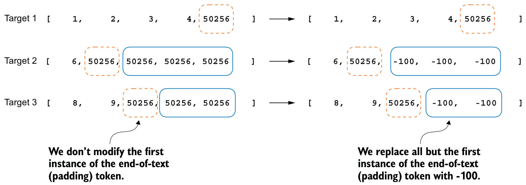
Applied to inputs_1 = [0, 1, 2, 3, 4], inputs_2 = [5, 6] and inputs_3 = [7, 8, 9], the function returns
tensor([[    0,     1,     2,     3,     4],
        [    5,     6, 50256, 50256, 50256],
        [    7,     8,     9, 50256, 50256]])
tensor([[    1,     2,     3,     4, 50256],
        [    6, 50256,  -100,  -100,  -100],
        [    8,     9, 50256,  -100,  -100]])
Why -100 is the value used
The chapter demonstrates the effect of -100 on three logit rows:
logits_2 = torch.tensor(
    [[-1.0, 1.0],
     [-0.5, 1.5],
     [-0.5, 1.5]]
)
targets_2 = torch.tensor([0, 1, 1])
loss_2 = torch.nn.functional.cross_entropy(logits_2, targets_2)
With the two-row logits and targets_1 = torch.tensor([0, 1]) the loss is 1.1269. Adding the third token gives 0.7936. Replacing the third target with -100, as targets_3 = torch.tensor([0, 1, -100]), returns the loss to tensor(1.1269), and loss_1 == loss_3 prints tensor(True). The default setting of the cross entropy function in PyTorch is cross_entropy(..., ignore_index=-100), so targets labeled -100 are dropped from the average entirely. Substituting any other out-of-range token ID raises an error instead.
Figure 7.13 shows the further option of replacing the instruction section of the target with -100, so the loss is computed only over the response and the model is not trained to reproduce instructions. Researchers are divided on whether this is universally beneficial. The 2024 paper by Shi et al., “Instruction Tuning With Loss Over Instructions” (https://arxiv.org/abs/2405.14394), demonstrated that not masking the instructions benefits LLM performance. The chapter does not apply instruction masking.
Learning outcomes
- dynamic-padding-collate-function Write a custom collate function that pads each batch to its own longest sequence.
- loss-masking-with-ignore-index Mask padding targets so they contribute nothing to the gradient.
Concepts
- custom-collate-function the function a
DataLoadercalls to merge samples into tensors, written here to pad per batch, slice shifted targets, apply the mask, and move the result to the device - loss-masking
-100is the defaultignore_indexof PyTorch cross entropy, so target positions carrying it are excluded from the loss average
Instruction data loaders
The device is chosen first, and the collate function receives it because the transfer happens inside collation rather than in the training loop:
device = torch.device("cuda" if torch.cuda.is_available() else "cpu")
# if torch.backends.mps.is_available():
#     device = torch.device("mps")
print("Device:", device)
Performing the device transfer inside the collate function makes it a background process outside the training loop, preventing it from blocking the GPU during model training. The two commented lines select an Apple Silicon GPU; the chapter notes that an "mps" device may produce numerical differences from the results printed in the text, as Apple Silicon support in PyTorch is still experimental.
custom_collate_fn takes five parameters, but a DataLoader calls its collate function with one argument. functools.partial fixes the rest:
from functools import partial

customized_collate_fn = partial(
    custom_collate_fn,
    device=device,
    allowed_max_length=1024
)
allowed_max_length=1024 truncates the data to the maximum context length supported by the GPT-2 model.
Listing 7.6 builds the three loaders. All use batch_size = 8, num_workers = 0 and customized_collate_fn; only the training loader shuffles and drops the final partial batch:
train_loader = DataLoader(
    train_dataset,
    batch_size=batch_size,
    collate_fn=customized_collate_fn,
    shuffle=True,
    drop_last=True,
    num_workers=num_workers
)
The validation and test loaders are constructed identically over val_dataset and test_dataset with shuffle=False and drop_last=False.
Printing inputs.shape, targets.shape for the training loader gives
Train loader:
torch.Size([8, 61]) torch.Size([8, 61])
torch.Size([8, 76]) torch.Size([8, 76])
torch.Size([8, 73]) torch.Size([8, 73])
...
torch.Size([8, 74]) torch.Size([8, 74])
torch.Size([8, 69]) torch.Size([8, 69])
The first dimension, 8, is the batch size. The second is the number of tokens in each training example in that batch — 61 for the first batch, 76 for the second. Inputs and targets always agree in shape, and the shape changes from batch to batch, which is the direct evidence that the padding is dynamic.
Learning outcomes
- dynamic-padding-collate-function Write a custom collate function that pads each batch to its own longest sequence.
- instruction-dataset-and-splits Load an instruction dataset, split it, and wrap it in a PyTorch Dataset.
Concepts
- custom-collate-function bound to a device and a maximum length with
functools.partial, it becomes the single-argument callable aDataLoaderexpects
Loading GPT-2 medium
Loading the pretrained weights uses the same code as pretraining and as the classification unit, with one substitution: "gpt2-medium (355M)" in place of "gpt2-small (124M)". The 124-million-parameter model is too limited in capacity to achieve satisfactory results via instruction fine-tuning; smaller models lack the necessary capacity to learn and retain the intricate patterns and nuanced behaviors required for high-quality instruction-following tasks.
Listing 7.7 gives the configuration:
BASE_CONFIG = {
    "vocab_size": 50257,     # Vocabulary size
    "context_length": 1024,  # Context length
    "drop_rate": 0.0,        # Dropout rate
    "qkv_bias": True         # Query-key-value bias
}

model_configs = {
    "gpt2-small (124M)": {"emb_dim": 768, "n_layers": 12, "n_heads": 12},
    "gpt2-medium (355M)": {"emb_dim": 1024, "n_layers": 24, "n_heads": 16},
    "gpt2-large (774M)": {"emb_dim": 1280, "n_layers": 36, "n_heads": 20},
    "gpt2-xl (1558M)": {"emb_dim": 1600, "n_layers": 48, "n_heads": 25},
}

CHOOSE_MODEL = "gpt2-medium (355M)"
BASE_CONFIG.update(model_configs[CHOOSE_MODEL])
The medium checkpoint occupies approximately 1.42 gigabytes, roughly three times the storage needed for the small model.
The baseline generation
Establishing what the model does before fine-tuning is what makes the later improvement attributable. The first validation example is formatted and generated from:
torch.manual_seed(123)
input_text = format_input(val_data[0])
print(input_text)
whose instruction is Convert the active sentence to passive: 'The chef cooks the meal every day.' Generation reuses the generate function from pretraining:
token_ids = generate(
    model=model,
    idx=text_to_token_ids(input_text, tokenizer),
    max_new_tokens=35,
    context_size=BASE_CONFIG["context_length"],
    eos_id=50256,
)
generated_text = token_ids_to_text(token_ids, tokenizer)
generate returns the combined input and output text, so the prompt is removed by slicing at its length: response_text = generated_text[len(input_text):].strip(). The output is
### Response:

The chef cooks the meal every day.

### Instruction:

Convert the active sentence to passive: 'The chef cooks the
The base model produces a ### Response: section, so it has learned the shape of the template from its pretraining corpus. What it writes into that section is the original input sentence and then part of the instruction again. It does not convert the sentence to passive voice.
Learning outcomes
- choosing-model-capacity Justify the choice of GPT-2 Medium over GPT-2 Small for instruction following.
- instruction-tuning-versus-base-pretraining Explain why a pretrained base LLM cannot follow instructions and what instruction fine-tuning changes.
Fine-tuning on instruction data
The loss function and training loop are imported unchanged from pretraining:
from chapter05 import (
    calc_loss_loader,
    train_model_simple
)
Measured over five batches with torch.no_grad(), the losses before training are
Training loss: 3.825908660888672
Validation loss: 3.7619335651397705
Listing 7.8 runs the fine-tuning:
import time

start_time = time.time()
torch.manual_seed(123)
optimizer = torch.optim.AdamW(
    model.parameters(), lr=0.00005, weight_decay=0.1
)
num_epochs = 2

train_losses, val_losses, tokens_seen = train_model_simple(
    model, train_loader, val_loader, optimizer, device,
    num_epochs=num_epochs, eval_freq=5, eval_iter=5,
    start_context=format_input(val_data[0]), tokenizer=tokenizer
)

end_time = time.time()
execution_time_minutes = (end_time - start_time) / 60
print(f"Training completed in {execution_time_minutes:.2f} minutes.")
Two details separate this from the classification unit. model.parameters() passes every parameter to the optimizer, where classification froze the backbone and trained only the last transformer block, the final LayerNorm and the new head. And start_context is a formatted prompt rather than a bare fragment, so the sample generated at each evaluation point can be read as an answer.
The printed progress begins and ends as
Ep 1 (Step 000000): Train loss 2.637, Val loss 2.626
Ep 1 (Step 000005): Train loss 1.174, Val loss 1.103
Ep 1 (Step 000010): Train loss 0.872, Val loss 0.944
Ep 1 (Step 000015): Train loss 0.857, Val loss 0.906
...
Ep 2 (Step 000230): Train loss 0.300, Val loss 0.657
Training completed in 0.87 minutes.
The sample generated at the end of training converts the active sentence "The chef cooks the meal every day." into "The meal is cooked every day by the chef." — the task the base model failed at in the previous section.
Two epochs is the whole schedule. The model demonstrated effective learning within these two epochs, so extending the training to a third epoch or more is not essential and may even be counterproductive, as it could lead to increased overfitting.
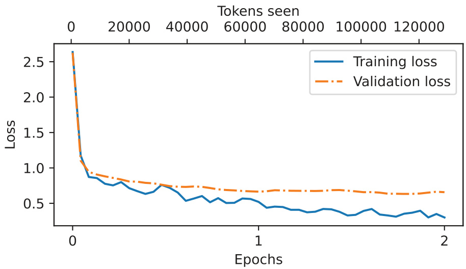
The rapid decrease during the initial phase indicates that the model quickly learns meaningful patterns and representations from the data. Through the second epoch the losses continue to decrease but at a slower rate, which indicates that the model is fine-tuning its learned representations and converging to a stable solution. The validation curve settles above the training curve and does not turn upward within the two epochs.
Reference run times for two epochs: gpt2-medium (355M) takes 15.78 minutes on an M3 MacBook Air CPU, 1.83 minutes on an NVIDIA L4 and 0.86 minutes on an A100. The same figures for gpt2-small (124M) are 5.74, 0.69 and 0.39 minutes.
Learning outcomes
- running-instruction-fine-tuning Fine-tune the model on instruction data and interpret the loss curves.
- loss-masking-with-ignore-index Mask padding targets so they contribute nothing to the gradient.
Concepts
- loss-masking the cross entropy minimized during these two epochs is averaged only over unmasked positions, so padding contributes no gradient
Extracting and saving responses
Listing 7.9 iterates the whole test set and attaches each generated response to its record:
from tqdm import tqdm

for i, entry in tqdm(enumerate(test_data), total=len(test_data)):
    input_text = format_input(entry)

    token_ids = generate(
        model=model,
        idx=text_to_token_ids(input_text, tokenizer).to(device),
        max_new_tokens=256,
        context_size=BASE_CONFIG["context_length"],
        eos_id=50256
    )
    generated_text = token_ids_to_text(token_ids, tokenizer)

    response_text = (
        generated_text[len(input_text):]
        .replace("### Response:", "")
        .strip()
    )
    test_data[i]["model_response"] = response_text

with open("instruction-data-with-response.json", "w") as file:
    json.dump(test_data, file, indent=4)
The extraction is two operations, not one. Slicing at len(input_text) removes the prompt that generate echoed back; .replace("### Response:", "") removes the header the model itself emitted. This is where the consistent template is repaid — the marker is a literal string, known in advance, identical in every record.
Processing the 110 test entries takes about 1 minute on an A100 GPU and 6 minutes on an M3 MacBook Air. A record then reads
{'instruction': 'Rewrite the sentence using a simile.',
 'input': 'The car is very fast.',
 'output': 'The car is as fast as lightning.',
 'model_response': 'The car is as fast as a bullet.'}
The weights are saved under a name derived from CHOOSE_MODEL:
import re

file_name = f"{re.sub(r'[ ()]', '', CHOOSE_MODEL) }-sft.pth"
torch.save(model.state_dict(), file_name)
print(f"Model saved as {file_name}")
The regular expression removes spaces and parentheses, giving gpt2-medium355M-sft.pth, which is reloaded with model.load_state_dict(torch.load("gpt2-medium355M-sft.pth")).
Reading three responses
Comparing the first three test records with their reference outputs shows the range of behavior.
The simile task is answered with “The car is as fast as a bullet.” against the reference “The car is as fast as lightning.”
A different simile, correctly formed. Open-ended tasks admit many correct answers, which is precisely why accuracy does not apply.
Asked what type of cloud is typically associated with thunderstorms, the model answers “a cumulus cloud” where the reference says “cumulonimbus”.
Close but not entirely accurate. Cumulus clouds can develop into cumulonimbus clouds, which are capable of producing thunderstorms.
Asked to name the author of Pride and Prejudice, the model answers “The author of ‘Pride and Prejudice’ is Jane Austen.” against the reference “Jane Austen.”
Correct, and more verbose than the reference. A string comparison would score this as a failure.
Learning outcomes
- extracting-and-saving-responses Generate responses over a test set and persist them for evaluation.
- alpaca-style-prompt-formatting Format instruction records into a consistent prompt template.
Concepts
- prompt-templates because
### Response:marks the boundary identically in every record, the generated answer can be isolated by a literal string operation
Evaluating with an LLM judge
Instruction-fine-tuned LLMs are evaluated by three families of method:
- Short-answer and multiple-choice benchmarks, such as Measuring Massive Multitask Language Understanding (MMLU, https://arxiv.org/abs/2009.03300), which test the general knowledge of a model.
- Human preference comparison to other LLMs, such as the LMSYS chatbot arena (https://lmsys.org).
- Automated conversational benchmarks, where another LLM such as GPT-4 is used to evaluate the responses, such as AlpacaEval (https://tatsu-lab.github.io/alpaca_eval/).
Human evaluation is laborious and time-consuming: reading and assigning ratings to all 1,100 responses would require a significant amount of effort. The chapter therefore implements the third family, using a custom test set rather than a public benchmark dataset so that the assessment is targeted at the intended use case.
Ollama runs the judge locally. It is a wrapper around the llama.cpp library, which implements LLMs in pure C/C++ to maximize efficiency, and it supports inference only — it does not support training or fine-tuning LLMs. The judge is the instruction-fine-tuned 8-billion-parameter Llama 3 model from Meta AI, downloaded by ollama run llama3, which occupies 4.7 GB of storage and requires approximately 16 GB of RAM.
For machines with less memory, the 3.8-billion-parameter phi3 model requires around 8 GB. For more powerful machines, llama3:70b is available at significantly greater computational cost.
Either the Ollama application or ollama serve must be running. A psutil check makes the requirement explicit rather than letting the REST calls fail:
ollama_running = check_if_running("ollama")

if not ollama_running:
    raise RuntimeError(
        "Ollama not running. Launch ollama before proceeding."
)
Listing 7.10 posts to the REST API. The options are what make the scoring reproducible:
    data = {
        "model": model,
        "messages": [
            {"role": "user", "content": prompt}
        ],
        "options": {
            "seed": 123,
            "temperature": 0,
            "num_ctx": 2048
        }
    }
with url="http://localhost:11434/api/chat" and model="llama3". The response arrives as a stream of lines, each a JSON object, and query_model accumulates response_json["message"]["content"] until an empty line ends the stream.
From critique to a number
Prompted with the input, the correct output and the model response, and asked to “score the model response … on a scale from 0 to 100, where 100 is the best score”, Llama 3 returns a paragraph of reasoning together with a score: 85 out of 100 for the bullet simile, 40 out of 100 for the cumulus cloud answer, and 95 out of 100 for the Jane Austen answer. The judge assigns partial credit where a response is not entirely correct.
Reasoning is not aggregable. Listing 7.11 appends one further instruction line, "Respond with the integer number only.", and converts the reply:
        score = query_model(prompt, model)
        try:
            scores.append(int(score))
        except ValueError:
            print(f"Could not convert score: {score}")
            continue
The try/except ValueError is not decoration: a judge is a language model, and a reply that is not parseable as an integer must be skipped rather than allowed to halt a run of 110 examples. Over the full test set,
Number of scores: 110 of 110
Average score: 50.32
The number is a benchmark for comparison against other models or against different training configurations, not an absolute measure of quality. For reference, under the same methodology the Llama 3 8B base model, without any fine-tuning, achieves an average score of 58.51 on the test set, and the Llama 3 8B instruct model achieves 82.6. Ollama is not entirely deterministic across operating systems, so the scores obtained may vary slightly; repeating the evaluation several times and averaging gives more robust results.
Learning outcomes
- llm-as-a-judge-evaluation Score open-ended responses automatically with a local LLM judge.
- extracting-and-saving-responses Generate responses over a test set and persist them for evaluation.
Concepts
- llm-as-a-judge a second, more capable model receives the instruction, the reference output and the response, and returns a 0–100 score that averages into one benchmark figure
- ollama a local wrapper around
llama.cppthat serves Llama 3 8B for inference over a REST API, keeping the evaluation reproducible and free of API costs
Where the field goes next
Figure 7.21 recapitulates the three stages: building an LLM, pretraining it into a foundation model, and fine-tuning that foundation model into either a classifier or a personal assistant.
Four directions extend the pipeline built here.
Preference fine-tuning. An optional step performed after instruction fine-tuning, particularly useful for customizing a model to better align with specific user preferences. Direct Preference Optimization is the method named, with code in the
04_preference-tuning-with-dpofolder of the book’s supplementary repository.Instruction fine-tuning learns from one reference answer per prompt. Preference fine-tuning learns from a comparison between candidate answers, which is what allows tone and style to be trained.
Parameter-efficient fine-tuning. Low-rank adaptation, LoRA, is offered as exercise 7.4: modify the code of this chapter to use the method from appendix E, then compare the training run time and model performance before and after the modification.
Configuration changes to the run itself. Four strategies are listed for improving performance: adjusting the hyperparameters during fine-tuning, such as the learning rate, batch size, or number of epochs; increasing the size of the training dataset or diversifying the examples to cover a broader range of topics and styles; experimenting with different prompts or instruction formats; and using a larger pretrained model.
Production frameworks. Axolotl (https://github.com/OpenAccess-AI-Collective/axolotl) and LitGPT (https://github.com/Lightning-AI/litgpt) implement these pipelines for real-world applications rather than for instruction.
Keeping current is done through recent research papers on arXiv at https://arxiv.org/list/cs.LG/recent, discussion on X and Reddit — the subreddit r/LocalLLaMA in particular — and technical blogs.
Learning outcomes
- next-steps-beyond-this-module Name the techniques and tools that extend fine-tuning beyond what we built.
Concepts
- instruction-fine-tuning supervised instruction fine-tuning is the last essential stage of the development cycle; preference fine-tuning and parameter-efficient methods build on top of it
The full arc completed
Instruction fine-tuning turns a base next-token predictor into a model that answers a request.
The objective does not change — it is next-token cross entropy throughout. What changes is that the training text is an instruction–response pair rendered in a fixed template.
Dynamic batch collation and target loss masking with
-100are what make instruction training correct and efficient.Padding to the longest sequence in each batch rather than the longest in the dataset avoids computing over mostly-padding tensors, and masking all but the first end-of-text token in each target keeps the stop signal while discarding the filler.
Parameter capacity is a design decision, not a default.
GPT-2 small (124M) sufficed for two-class classification. Instruction following requires holding a request in context and producing a structured response, and the 355M medium model is the smallest of the four configurations that does so within two epochs.
Automated evaluation with a local LLM judge yields a comparable number where accuracy does not apply.
An average of 50.32 across the 110 test responses is meaningful only against other numbers produced the same way — 58.51 for the Llama 3 8B base model, 82.6 for its instruct variant.
Every component of the pipeline was written by hand.
Tokenization, the attention mechanism, the transformer block, the training loop, the loss, and now the data pipeline and evaluation that turn a foundation model into an assistant.
References
- Building a Large Language Model (from scratch), Sebastian Raschka, 2024, Manning Books — Link — Page 226-272