Lecture notes — Chapter 12: Transformers
ver. 1.1.0, chapter_12_transformers
ver. 1.1.0 · 2026-09-02 16:27:37
Where this fits
This is the first unit of the module, so nothing precedes it. Two results from the convolutional material are used throughout. The first is parameter sharing: a convolutional layer applies the same weights at every position, which is what makes a network with a very large number of input variables trainable at all. The second is the residual connection and its normalization layer, which is what permits a stack of many layers to be optimized.
Text does not sit on a regular grid. A convolutional layer shares parameters across positions but its connections are fixed by its weights, and the connections text needs depend on the words themselves. Dot-product self-attention supplies exactly that: a layer whose connections are computed from the data. Every model in the remainder of this module — BERT, GPT3, and the language model built from scratch in the later units — is a stack of layers built around it.
Understanding Deep Learning, Simon Prince, 2026, chapter 12. Chapter 10 of the same book is the convolutional material referred to above.
Learning outcomes
motivate-attention-for-sequences— Explain why fully connected networks and convolutional networks are poorly suited to text, and what properties self-attention supplies instead.compute-dot-product-self-attention— Compute dot-product self-attention from queries, keys and values, in both per-token and matrix form.apply-attention-extensions— Apply positional encoding, dot-product scaling, and multiple heads to make self-attention usable in practice.assemble-transformer-layer— Assemble a transformer layer from multi-head self-attention, a position-wise MLP, residual connections and LayerNorm.prepare-text-for-transformers— Turn raw text into the input a transformer consumes, using sub-word tokenization and learned embeddings.contrast-transformer-paradigms— Distinguish encoder, decoder and encoder-decoder transformers by their attention masking and their training objective.analyze-attention-complexity— Analyse the quadratic cost of full self-attention and describe the main strategies that reduce it.adapt-transformers-to-images— Describe how transformers are adapted to images by treating patches or pixels as tokens.
Concepts introduced
- Dot-product self-attention — each output is a weighted sum of value vectors computed from all inputs, with the weights given by a softmax over query-key dot products.
- Scaled dot-product attention — the same mechanism with the dot products divided by \(\sqrt{D_q}\), so the softmax does not saturate.
- Multi-head attention — \(H\) self-attention mechanisms applied in parallel on projections of size \(D/H\), concatenated and recombined by a linear transform \(\boldsymbol\Omega_c\).
- Positional encoding — position information supplied either by a matrix \(\boldsymbol\Pi\) added to the input, or by a learned parameter per relative offset added to the attention matrix.
- Transformer layer — multi-head self-attention and a token-wise MLP, each in a residual block, each followed by LayerNorm.
- Sub-word tokenization — a vocabulary built by greedily merging the most frequent adjacent token pair, halting at a chosen vocabulary size.
- Masked self-attention — dot products for future positions set to negative infinity before the softmax, so position \(n\) attends only to positions up to \(n\).
- Cross-attention — queries from the decoder embeddings, keys and values from the encoder embeddings.
- Sparse and efficient attention — local, dilated and global-token interaction patterns, low-rank key/value projection, and kernel rewrites, all aimed at the \(O(N^2)\) cost.
- Vision Transformer — an encoder applied to \(16\times16\) image patches projected to token embeddings, with a
<cls>token for classification. - Multi-scale vision transformers — attention within local windows, shifted in alternate layers, with patch merging between resolutions.
What makes text hard
Consider the passage the chapter uses to motivate the architecture:
The restaurant refused to serve me a ham sandwich because it only cooks vegetarian food. In the end, they just gave me two slices of bread. Their ambiance was just as good as the food and service.
The goal is a network that turns this text into a representation suitable for downstream tasks, such as classifying the review as positive or negative, or answering “Does the restaurant serve steak?”. Three observations follow from the passage itself.
The encoded input is large. Each of the 37 words might be represented by an embedding vector of length 1024, so the encoded input has length \(37 \times 1024 = 37888\).
A realistically sized body of text has hundreds or thousands of words, so a fully connected network over the whole passage is impractical.
Each input is of a different length. One input may be a sentence, another many sentences. It is not obvious how to apply a fully connected network at all, since the weight matrix would have to change with the length.
These first two observations together suggest sharing parameters across words at different input positions, in the way that a convolutional network shares parameters across image positions.
Language is ambiguous. It is not clear from the syntax alone that the pronoun it refers to the restaurant and not to the ham sandwich. To understand the text, the word it must somehow be connected to the word restaurant.
In the parlance of transformers, the former word should pay attention to the latter. The strength of such a connection must depend on the words themselves, and the connection must reach across large text spans — the word their in the last sentence also refers to the restaurant.
The two requirements are therefore parameter sharing, to cope with long passages of differing lengths, and connections between word representations whose strength depends on the words. Both are properties of the layer, not of the data, and the transformer acquires them by using dot-product self-attention.
An image of the wrong size can be rescaled to the network’s input size, because the statistics of an image are approximately unchanged by resampling. A text sequence has no comparable operation: there is no way to resize a forty-word passage to twenty words without deleting words. Variable length is therefore a permanent property of the input, not a preprocessing inconvenience.
Learning outcomes
- motivate-attention-for-sequences Explain why fully connected networks and convolutional networks are poorly suited to text, and what properties self-attention supplies instead.
Dot-product self-attention
A standard neural network layer \(\mathbf{f}[\mathbf{x}]\) takes a \(D \times 1\) input \(\mathbf{x}\) and applies a linear transformation followed by an activation function like a ReLU:
\[\mathbf{f}[\mathbf{x}] = \text{ReLU}[\boldsymbol\beta + \boldsymbol\Omega\mathbf{x}]\]
A self-attention block \(\mathbf{sa}[\bullet]\) takes \(N\) inputs \(\mathbf{x}_1, \ldots, \mathbf{x}_N\), each of dimension \(D \times 1\), and returns \(N\) outputs, each also of size \(D \times 1\). It has two halves that meet at the end.
The values, and their weighting
A set of values is computed for each input:
\[\mathbf{v}_m = \boldsymbol\beta_v + \boldsymbol\Omega_v\mathbf{x}_m\]
where \(\boldsymbol\beta_v \in \mathbb{R}^{D \times 1}\) and \(\boldsymbol\Omega_v \in \mathbb{R}^{D \times D}\). The \(n^{th}\) output is a weighted sum of all the values:
\[\mathbf{sa}_n[\mathbf{x}_1, \ldots, \mathbf{x}_N] = \sum_{m=1}^{N} a[\mathbf{x}_m, \mathbf{x}_n]\mathbf{v}_m\]
The scalar weight \(a[\mathbf{x}_m, \mathbf{x}_n]\) is the attention that the \(n^{th}\) output pays to input \(\mathbf{x}_m\). The \(N\) weights \(a[\bullet, \mathbf{x}_n]\) are non-negative and sum to one, so self-attention can be thought of as routing the values in different proportions to create each output.
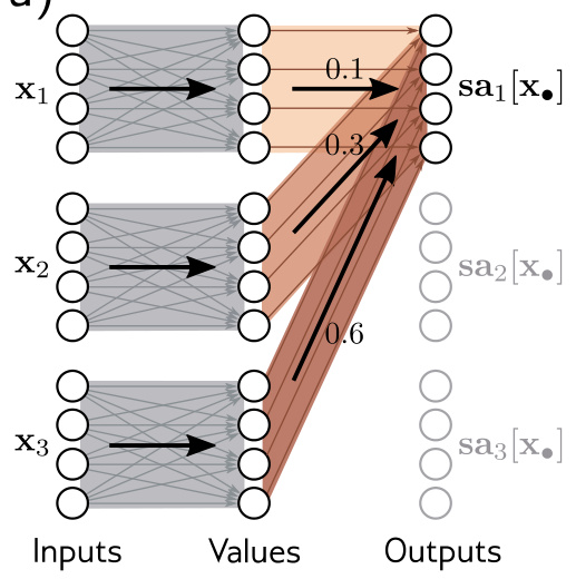
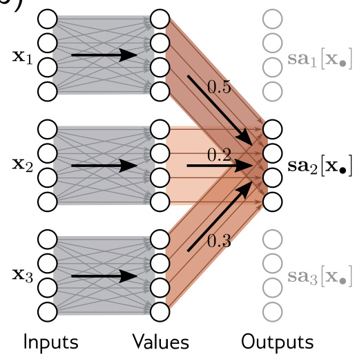
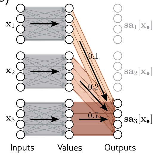
The same weights \(\boldsymbol\Omega_v\) and biases \(\boldsymbol\beta_v\) are applied to every input, so the value computation scales linearly with the sequence length \(N\) and needs fewer parameters than a fully connected network relating all \(DN\) inputs to all \(DN\) values. The attention weights are also sparse in a specific sense: there is only one weight for each ordered pair of inputs \((\mathbf{x}_m, \mathbf{x}_n)\), regardless of the size of those inputs. The number of attention weights therefore has a quadratic dependence on \(N\), and is independent of the length \(D\) of each input.
The attention weights
Two more linear transformations of the inputs give the queries and the keys:
\[\mathbf{q}_n = \boldsymbol\beta_q + \boldsymbol\Omega_q\mathbf{x}_n, \qquad \mathbf{k}_m = \boldsymbol\beta_k + \boldsymbol\Omega_k\mathbf{x}_m\]
The attention weights are the softmax over \(m\) of the dot products between the query and the keys:
\[a[\mathbf{x}_m, \mathbf{x}_n] = \text{softmax}_m\!\left[\mathbf{k}_\bullet^T\mathbf{q}_n\right] = \frac{\exp\!\left[\mathbf{k}_m^T\mathbf{q}_n\right]}{\sum_{m'=1}^{N}\exp\!\left[\mathbf{k}_{m'}^T\mathbf{q}_n\right]}\]
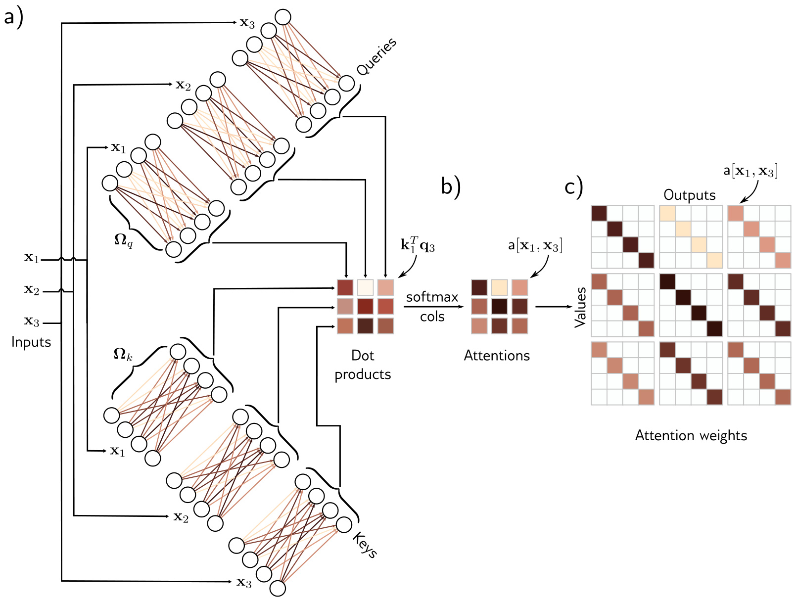
The names come from information retrieval. The dot product is a measure of similarity between its inputs, so the weights \(a[\bullet, \mathbf{x}_n]\) depend on the relative similarities between the \(n^{th}\) query and all of the keys. The softmax means the key vectors compete with one another to contribute to the final result. Queries and keys must have the same dimension, but that dimension can differ from the dimension of the values, which is usually the same size as the input so that the representation does not change size.
The mechanism is nonlinear even though both of its halves are linear maps. The values are computed independently for each input and combined linearly, but the weights are themselves nonlinear functions of the input. This makes self-attention an example of a hypernetwork, in which one branch of a network computes the weights of another.
Learning outcomes
- compute-dot-product-self-attention Compute dot-product self-attention from queries, keys and values, in both per-token and matrix form.
Concepts
- dot-product-self-attention value vectors \(\mathbf{v}_m = \boldsymbol\beta_v + \boldsymbol\Omega_v\mathbf{x}_m\) are computed once per position and combined by softmax-normalized query-key dot products
Self-attention in matrix form
The \(n^{th}\) output is a weighted sum of the same linear transformation \(\mathbf{v}_\bullet = \boldsymbol\beta_v + \boldsymbol\Omega_v\mathbf{x}_\bullet\) applied to all of the inputs, where the weights are positive and sum to one, and depend on a measure of similarity between input \(\mathbf{x}_n\) and the other inputs. There is no activation function.
Two properties follow, and they are the reason the mechanism was wanted.
There is a single shared set of parameters \(\boldsymbol\phi = \{\boldsymbol\beta_v, \boldsymbol\Omega_v, \boldsymbol\beta_q, \boldsymbol\Omega_q, \boldsymbol\beta_k, \boldsymbol\Omega_k\}\).
This is independent of the number of inputs \(N\), so the network can be applied to different sequence lengths.
There are connections between the inputs, and the strength of these connections depends on the inputs themselves via the attention weights.
This is what allows the word it to be connected to the word restaurant rather than to a fixed position.
The computation is written compactly if the \(N\) inputs \(\mathbf{x}_n\) form the columns of the \(D \times N\) matrix \(\mathbf{X}\). The values, queries and keys are then
\[\mathbf{V}[\mathbf{X}] = \boldsymbol\beta_v\mathbf{1}^T + \boldsymbol\Omega_v\mathbf{X}, \quad \mathbf{Q}[\mathbf{X}] = \boldsymbol\beta_q\mathbf{1}^T + \boldsymbol\Omega_q\mathbf{X}, \quad \mathbf{K}[\mathbf{X}] = \boldsymbol\beta_k\mathbf{1}^T + \boldsymbol\Omega_k\mathbf{X}\]
where \(\mathbf{1}\) is an \(N \times 1\) vector containing ones. The self-attention computation is then
\[\mathbf{Sa}[\mathbf{X}] = \mathbf{V}[\mathbf{X}] \cdot \mathbf{Softmax}\!\left[\mathbf{K}[\mathbf{X}]^T\mathbf{Q}[\mathbf{X}]\right]\]
where \(\mathbf{Softmax}[\bullet]\) takes a matrix and performs the softmax operation independently on each of its columns. The dependence on \(\mathbf{X}\) is written explicitly here to emphasize that self-attention computes a kind of triple product based on the inputs. From here on it is dropped:
\[\mathbf{Sa}[\mathbf{X}] = \mathbf{V} \cdot \mathbf{Softmax}\!\left[\mathbf{K}^T\mathbf{Q}\right]\]
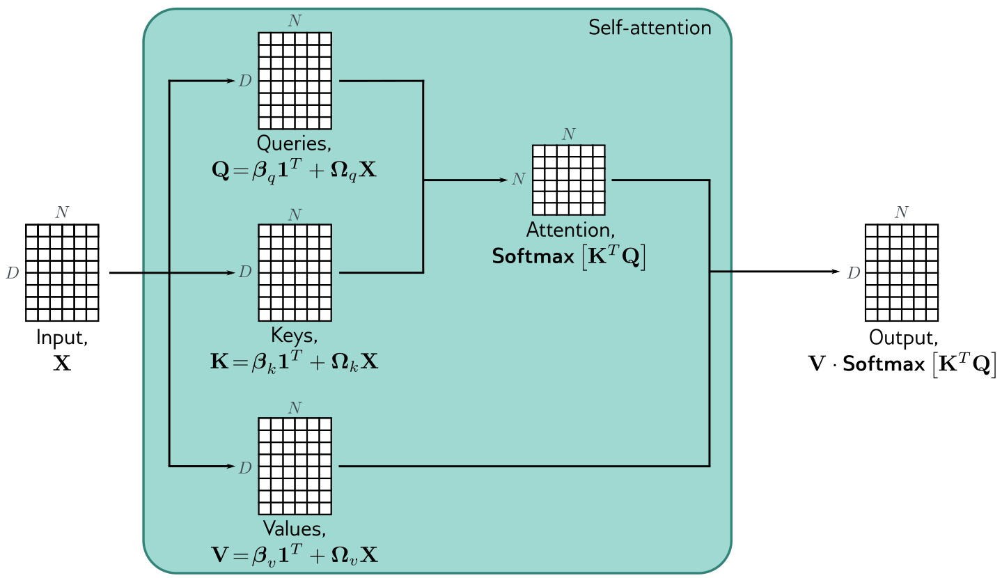
Two consequences of this form should be read off now, because each motivates a later section. The softmax is applied column-wise, so each column of the attention matrix sums to one and every output is a convex combination of the values. And the attention matrix \(\mathbf{K}^T\mathbf{Q}\) is \(N \times N\): its size is quadratic in the sequence length.
Every operation in the expression is a matrix multiplication or a column-wise softmax. Both parallelize across the sequence, so the whole layer executes as four matrix products and one elementwise nonlinearity, with no loop over positions.
Learning outcomes
- compute-dot-product-self-attention Compute dot-product self-attention from queries, keys and values, in both per-token and matrix form.
Concepts
- dot-product-self-attention the whole layer is \(\mathbf{Sa}[\mathbf{X}] = \mathbf{V} \cdot \mathbf{Softmax}[\mathbf{K}^T\mathbf{Q}]\), computed from one parameter set shared across all \(N\) positions
Three extensions used in practice
Three modifications to the mechanism above are almost always used.
Positional encoding
The computation does not take into account the order of the inputs \(\mathbf{x}_n\). More precisely, it is equivariant with respect to input permutations: for any permutation matrix \(\mathbf{P}\),
\[\mathbf{Sa}[\mathbf{X}\mathbf{P}] = \mathbf{Sa}[\mathbf{X}]\mathbf{P}\]
Order is important when the inputs correspond to words in a sentence. The sentence The woman ate the raccoon has a different meaning than The raccoon ate the woman, yet the two produce the same set of outputs in a different order. There are two main approaches to incorporating position information.
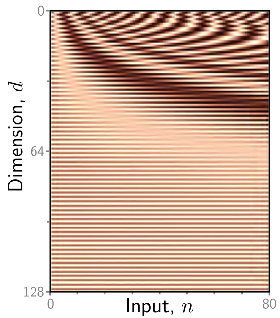
Absolute positional encodings. A matrix \(\boldsymbol\Pi\) is added to the input \(\mathbf{X}\). Each column of \(\boldsymbol\Pi\) is unique and hence contains information about the absolute position in the input sequence. This matrix can be chosen by hand or learned. It may be added to the network inputs or at every network layer, and is sometimes added to \(\mathbf{X}\) in the computation of the queries and keys but not to the values.
Relative positional encodings. The absolute position of a word is much less important than the relative position between two words, since the input may be a whole sentence or just a fragment. Each element of the attention matrix corresponds to a particular offset between key position \(a\) and query position \(b\). A parameter \(\pi_{a,b}\) is learned for each offset and used to modify the attention matrix, by adding these values, multiplying by them, or altering the matrix in some other way.
Scaled dot-product self-attention
The dot products in the attention computation can have large magnitudes and move the arguments to the softmax function into a region where the largest value completely dominates. Small changes to the inputs to the softmax then have little effect on the output, so the gradients are very small and the model is difficult to train. To prevent this, the dot products are scaled by the square root of the dimension \(D_q\) of the queries and keys — the number of rows in \(\boldsymbol\Omega_q\) and \(\boldsymbol\Omega_k\), which must be the same:
\[\mathbf{Sa}[\mathbf{X}] = \mathbf{V} \cdot \mathbf{Softmax}\!\left[\frac{\mathbf{K}^T\mathbf{Q}}{\sqrt{D_q}}\right]\]
Multiple heads
Multiple self-attention mechanisms are usually applied in parallel, which is known as multi-head self-attention. Now \(H\) different sets of values, keys and queries are computed,
\[\mathbf{V}_h = \boldsymbol\beta_{vh}\mathbf{1}^T + \boldsymbol\Omega_{vh}\mathbf{X}, \quad \mathbf{Q}_h = \boldsymbol\beta_{qh}\mathbf{1}^T + \boldsymbol\Omega_{qh}\mathbf{X}, \quad \mathbf{K}_h = \boldsymbol\beta_{kh}\mathbf{1}^T + \boldsymbol\Omega_{kh}\mathbf{X}\]
and the \(h^{th}\) self-attention mechanism, or head, is
\[\mathbf{Sa}_h[\mathbf{X}] = \mathbf{V}_h \cdot \mathbf{Softmax}\!\left[\frac{\mathbf{K}_h^T\mathbf{Q}_h}{\sqrt{D_q}}\right]\]
Typically, if the dimension of the inputs \(\mathbf{x}_m\) is \(D\) and there are \(H\) heads, the values, queries and keys are all of size \(D/H\), which allows for an efficient implementation. The outputs are vertically concatenated and another linear transform \(\boldsymbol\Omega_c\) is applied to combine them:
\[\mathbf{MhSa}[\mathbf{X}] = \boldsymbol\Omega_c\!\left[\mathbf{Sa}_1[\mathbf{X}]^T, \mathbf{Sa}_2[\mathbf{X}]^T, \ldots, \mathbf{Sa}_H[\mathbf{X}]^T\right]^T\]
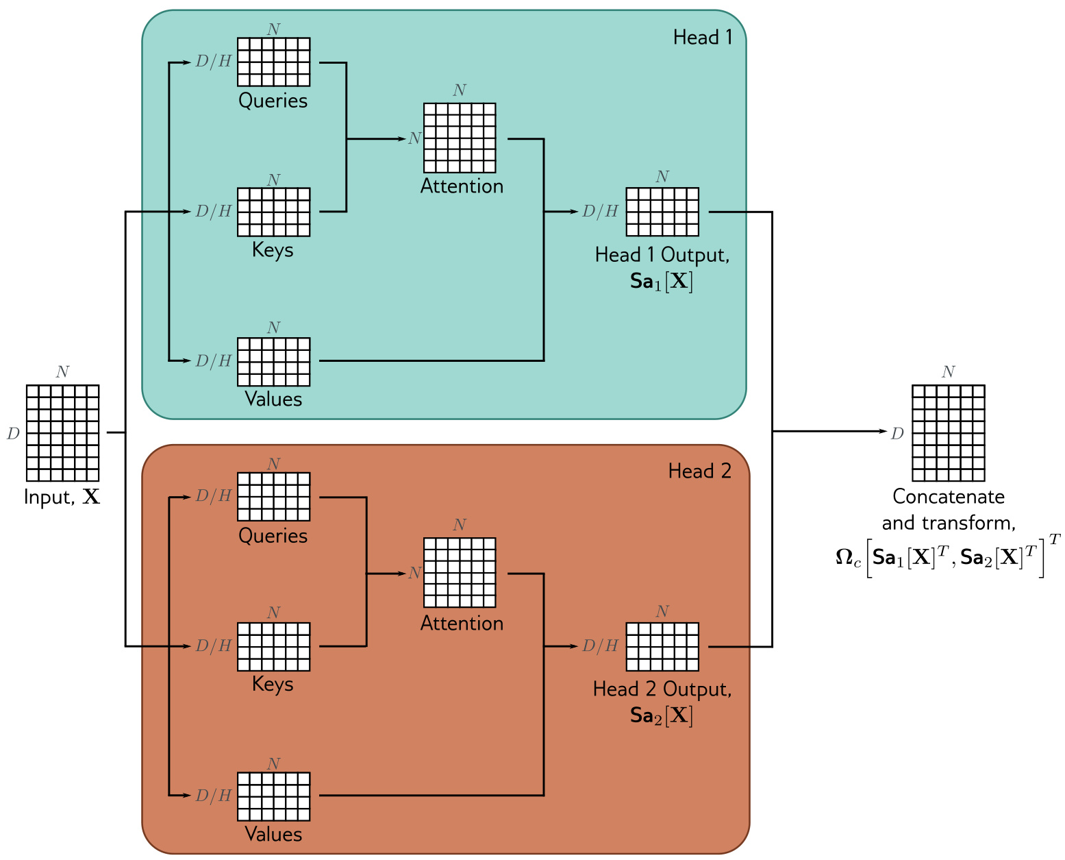
Multiple heads seem to be necessary to make self-attention work well. It has been speculated that they make the self-attention network more robust to bad initializations.
Key ideas
- Permutation equivariance, \(\mathbf{Sa}[\mathbf{X}\mathbf{P}] = \mathbf{Sa}[\mathbf{X}]\mathbf{P}\), is a property of the mechanism, so order must be supplied from outside it.
- Absolute encodings add a distinct column per position; relative encodings learn one parameter per query-key offset.
- Scaling by \(\sqrt{D_q}\) addresses a gradient problem, not an accuracy problem: the unscaled softmax saturates and stops learning.
- Setting each head’s dimension to \(D/H\) keeps the parameter count and computation of \(H\) heads comparable to one head of dimension \(D\).
Learning outcomes
- apply-attention-extensions Apply positional encoding, dot-product scaling, and multiple heads to make self-attention usable in practice.
Concepts
- positional-encoding a distinct vector per absolute position added to the input, or a learned parameter per relative offset applied to the attention matrix
- scaled-dot-product-attention dividing the query-key dot products by \(\sqrt{D_q}\) keeps the softmax out of the region where the largest value dominates and the gradients vanish
- dot-product-self-attention the scaled form \(\mathbf{V} \cdot \mathbf{Softmax}[\mathbf{K}^T\mathbf{Q}/\sqrt{D_q}]\) is the version used in practice
- multi-head-attention \(H\) heads with values, queries and keys of size \(D/H\) are evaluated in parallel, concatenated vertically and recombined by \(\boldsymbol\Omega_c\)
The transformer layer
Self-attention is just one part of a larger transformer layer. This consists of a multi-head self-attention unit, which allows the word representations to interact with each other, followed by a fully connected network \(\mathbf{mlp}[\mathbf{x}_\bullet]\) that operates separately on each word. Both units are residual networks, so their output is added back to the original input. In addition, it is typical to add a LayerNorm operation after both the self-attention and fully connected networks. LayerNorm is similar to BatchNorm, but normalizes each embedding in each batch element separately using statistics calculated across its \(D\) embedding dimensions.
The complete layer is the following series of operations:
\[ \begin{aligned} \mathbf{X} &\leftarrow \mathbf{X} + \mathbf{MhSa}[\mathbf{X}] \\ \mathbf{X} &\leftarrow \mathbf{LayerNorm}[\mathbf{X}] \\ \mathbf{x}_n &\leftarrow \mathbf{x}_n + \mathbf{mlp}[\mathbf{x}_n] \qquad \forall\, n \in \{1, \ldots, N\} \\ \mathbf{X} &\leftarrow \mathbf{LayerNorm}[\mathbf{X}] \end{aligned} \]
where the column vectors \(\mathbf{x}_n\) are separately taken from the full data matrix \(\mathbf{X}\). In a real network, the data passes through a series of these transformer layers.
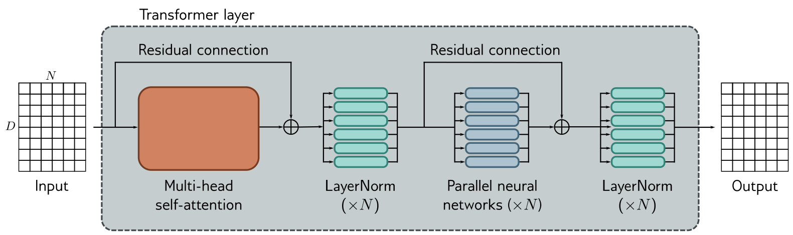
The division of labour between the two halves is the point of the block.
Multi-head self-attention moves information between positions. It is the only operation in the layer that lets one token’s representation depend on another’s.
This is also why masking the attention matrix, and nothing else, is sufficient to make a decoder causal — the tokens only interact in the self-attention layers.
The MLP processes information within a position. The same fully connected network is applied separately to each of the \(N\) word representations, which supplies the nonlinearity that self-attention itself lacks.
Because it is applied per column, it is indifferent to the sequence length, so the layer as a whole retains the property that let self-attention accept any \(N\).
Training transformers requires learning rate warm-up and Adam. Gradients vanish without warm-up; placing the LayerNorm outside the residual block causes gradients to shrink as they pass back through the network, and the gradients for the query and key parameters are smaller than those for the value parameters.
Learning outcomes
- assemble-transformer-layer Assemble a transformer layer from multi-head self-attention, a position-wise MLP, residual connections and LayerNorm.
From text to tokens to embeddings
Everything above assumed an input matrix \(\mathbf{X}\) of embeddings. A typical NLP pipeline produces it in two stages: a tokenizer splits the text into words or word fragments, and each token is mapped to a learned embedding.
Tokenization
A tokenizer splits text into smaller constituent units, called tokens, drawn from a vocabulary of possible tokens. Taking the tokens to be words has three difficulties.
- Inevitably, some words, such as names, will not be in the vocabulary.
- It is unclear how to handle punctuation, but this is important: if a sentence ends in a question mark, that information must be encoded.
- The vocabulary would need different tokens for versions of the same word with different suffixes — walk, walks, walked, walking — and there is no way to clarify that these variations are related.
Using letters and punctuation marks as the vocabulary avoids all three, but means splitting text into very small parts and requiring the subsequent network to re-learn the relations between them. In practice a compromise between letters and full words is used. The vocabulary is computed using a sub-word tokenizer such as byte pair encoding, which greedily merges commonly occurring sub-strings based on their frequency.
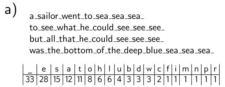

At each iteration the tokenizer finds the most commonly occurring adjacent pair of tokens and merges them. In the worked example, the first merge is se, which decreases the counts for the original tokens s and e; the second merges e with the whitespace character. The last character of the first token to be merged cannot be whitespace, which prevents merging across words. Continued indefinitely, the tokens eventually represent full words; in practice the algorithm terminates when the vocabulary size reaches a predetermined value. The number of tokens first increases as word fragments are added to the letters, then decreases again as those fragments merge into words.
Embeddings
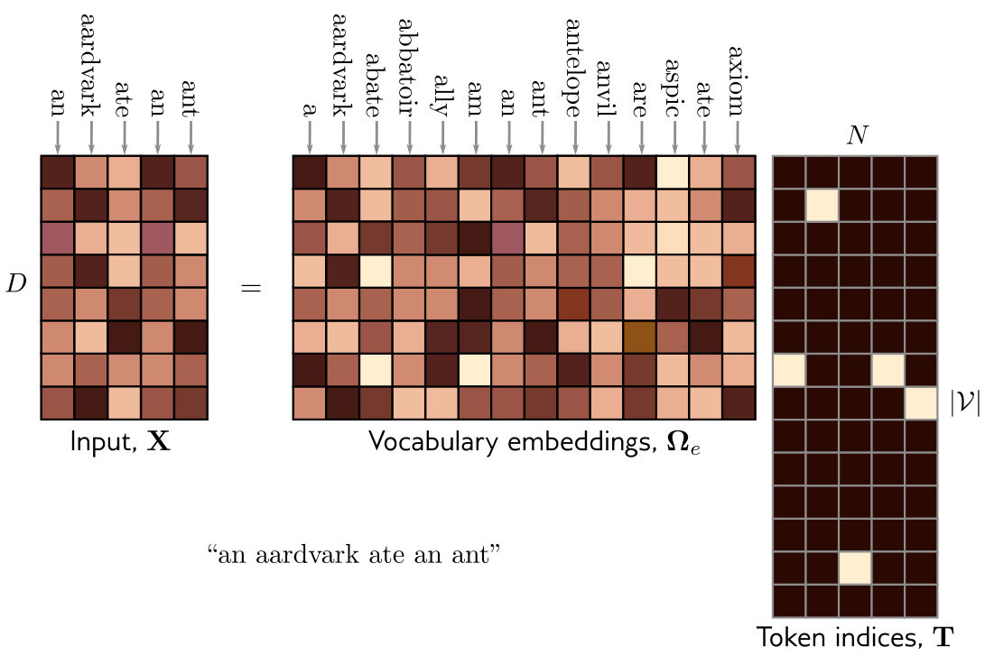
Each token in the vocabulary \(\mathcal{V}\) is mapped to a unique word embedding, and the embeddings for the whole vocabulary are stored in a matrix \(\boldsymbol\Omega_e \in \mathbb{R}^{D \times |\mathcal{V}|}\). The \(N\) input tokens are first encoded in the matrix \(\mathbf{T} \in \mathbb{R}^{|\mathcal{V}| \times N}\), where the \(n^{th}\) column corresponds to the \(n^{th}\) token and is a \(|\mathcal{V}| \times 1\) one-hot vector: every entry is zero except the entry corresponding to the token, which is set to one. The input embeddings are computed as
\[\mathbf{X} = \boldsymbol\Omega_e\mathbf{T}\]
and \(\boldsymbol\Omega_e\) is learned like any other network parameter. A typical embedding size \(D\) is 1024 and a typical total vocabulary size \(|\mathcal{V}|\) is 30,000, so even before the main network there are many parameters in \(\boldsymbol\Omega_e\) to learn.
Transformer model
Finally, the embedding matrix \(\mathbf{X}\) representing the text is passed through a series of \(K\) transformer layers, called a transformer model. There are three types. An encoder transforms the text embeddings into a representation that can support a variety of tasks. A decoder predicts the next token to continue the input text. Encoder-decoders are used in sequence-to-sequence tasks, where one text string is converted into another.
The embedding of a token depends only on its index, so two occurrences of the same word enter the network as the same vector. Everything that distinguishes them — their position, and their context — is supplied later, by the positional encoding and by the attention layers.
Learning outcomes
- prepare-text-for-transformers Turn raw text into the input a transformer consumes, using sub-word tokenization and learned embeddings.
Concepts
- sub-word-tokenization byte pair encoding greedily merges the most frequent adjacent token pair, halting at a chosen vocabulary size, so frequent whole words and shared fragments coexist
- transformer-layer a transformer model is \(K\) such layers stacked, and the stack is an encoder, a decoder or an encoder-decoder according to how attention is arranged
Encoder models: BERT
BERT is an encoder model that uses a vocabulary of 30,000 tokens. Input tokens are converted to 1024-dimensional word embeddings and passed through 24 transformer layers. Each contains a self-attention mechanism with 16 heads. The queries, keys and values for each head are of dimension 64, so the matrices \(\boldsymbol\Omega_{vh}, \boldsymbol\Omega_{qh}, \boldsymbol\Omega_{kh}\) are \(64 \times 1024\). The dimension of the single hidden layer in the fully connected networks is 4096. The total number of parameters is around 340 million.
Encoder models like BERT exploit transfer learning. During pre-training, the parameters of the transformer architecture are learned using self-supervision from a large corpus of text, so that the model learns general information about the statistics of language. In the fine-tuning stage, the resulting network is adapted to solve a particular task using a smaller body of labelled training data.
Pre-training
The self-supervision task consists of predicting missing words from sentences in a large internet corpus. A small fraction of the input tokens are randomly replaced with a generic <mask> token, the outputs corresponding to the masked tokens are passed through softmax functions, and a multiclass classification loss is applied to each. During training the maximum input length is 512 tokens and the batch size is 256. The system is trained for a million steps, corresponding to roughly 50 epochs of the 3.3-billion word corpus.
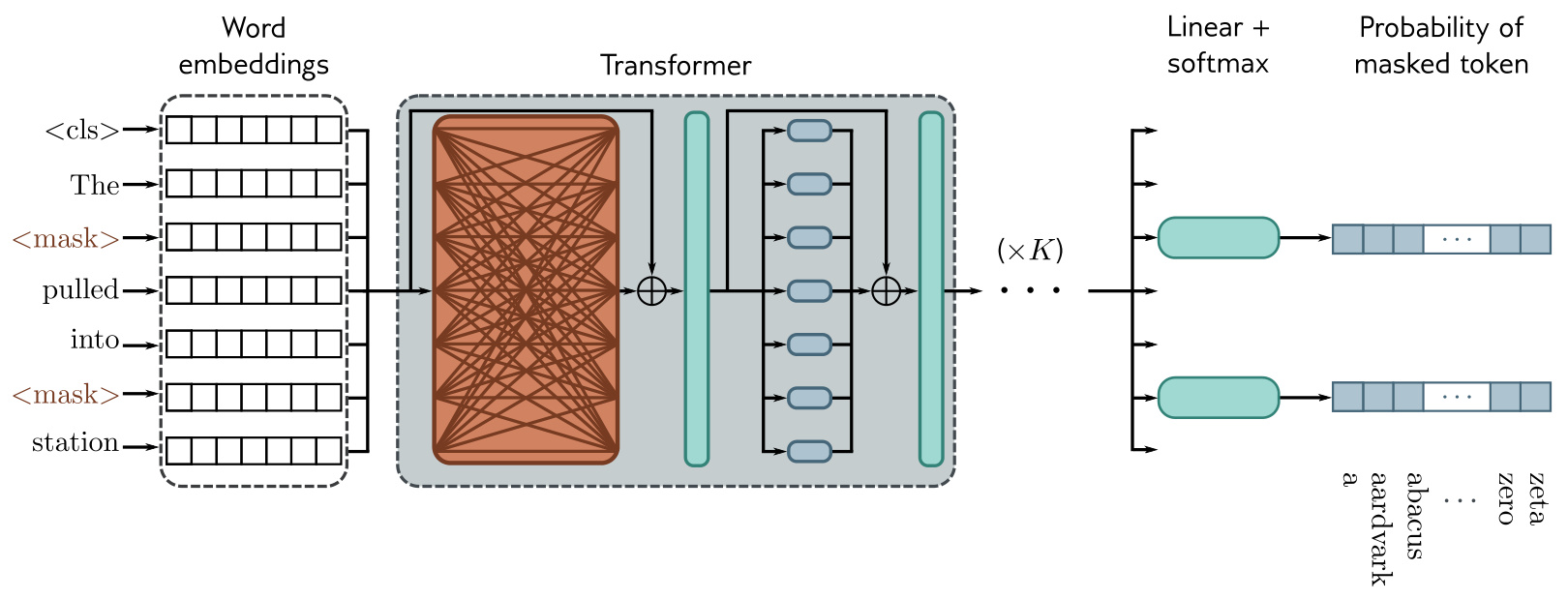
<cls> token denoting the start of the sequence, are converted to word embeddings and passed through the transformer layers; orange connections indicate that every token attends to every other token.Predicting missing words forces the network to understand some syntax. It might learn that the adjective red is often found before nouns like house or car but never before a verb like shout. It also allows the model to learn superficial common sense about the world: after training, the model assigns a higher probability to the missing word train in the sentence The <mask> pulled into the station than it would to the word peanut.
The task uses both the left and right context to predict the missing word, which is the advantage of unmasked attention. Its disadvantage is that it does not make efficient use of data: in the figure, seven tokens are processed to add two terms to the loss function.
Fine-tuning
An extra layer is appended onto the transformer network to convert the output vectors to the desired output format.
- Text classification. The vector associated with the
<cls>token, which is placed at the start of every string during pre-training, is mapped to a single number and passed through a logistic sigmoid, contributing to a binary cross-entropy loss. - Word classification. For named entity recognition, each input embedding \(\mathbf{x}_n\) is mapped to an \(E \times 1\) vector where the \(E\) entries correspond to the \(E\) entity types, and a softmax gives a multiclass cross-entropy loss.
- Text span prediction. In the SQuAD 1.1 question answering task, the question and a passage from Wikipedia containing the answer are concatenated and tokenized. Each token maps to two numbers indicating how likely it is that the answer span begins and ends at that location; two softmax functions are applied, and the likelihood of any span is derived by combining the probability of starting and ending at the appropriate places.
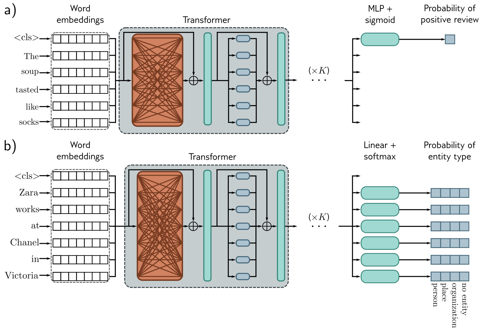
<cls> embedding, and for named entity recognition from each word’s embedding.Learning outcomes
- contrast-transformer-paradigms Distinguish encoder, decoder and encoder-decoder transformers by their attention masking and their training objective.
Concepts
- transformer-layer BERT stacks 24 of these layers with 16 heads each, and the whole stack is pre-trained by predicting masked tokens
Decoder models: GPT3
The basic architecture of a decoder is extremely similar to the encoder: a series of transformer layers that operate on learned word embeddings. The goal is different. The encoder builds a representation of the text that can be fine-tuned for a variety of NLP tasks; the decoder has one purpose, to generate the next token in a sequence.
Language modeling
GPT3 is an autoregressive language model. For the sentence It takes great courage to let yourself appear weak, taking the tokens to be full words, the probability of the full sentence factors as
\[ \begin{aligned} Pr(\text{It takes great courage to let yourself appear weak}) = \\ Pr(\text{It}) \times Pr(\text{takes}|\text{It}) \times Pr(\text{great}|\text{It takes}) \times \cdots \end{aligned} \]
with one factor per token, each conditioned on all the words before it. An autoregressive model predicts the conditional distributions \(Pr(t_n|t_1, \ldots, t_{n-1})\) of each token given all the prior tokens, and hence indirectly computes the joint probability of all \(N\) tokens:
\[Pr(t_1, t_2, \ldots, t_N) = Pr(t_1)\prod_{n=2}^{N} Pr(t_n|t_1, \ldots, t_{n-1})\]
This is the connection between maximizing the joint probability of the tokens and the next token prediction task.
Masked self-attention
Training seeks parameters that maximize the log probability of the input text under the autoregressive model. Ideally the whole sentence is passed in and all the log probabilities and gradients are computed in the same forward pass. But if the full sentence is passed in, the term computing \(\log[Pr(\text{great}|\text{It takes})]\) would have access to both the answer great and the right context courage to let yourself appear weak. The system can then cheat rather than learn to predict the following words, and will not train properly.
The tokens only interact in the self-attention layers, so the problem is resolved by ensuring that the attention to the answer and the right context is zero. This is achieved by setting the corresponding dot products in the self-attention computation to negative infinity before they are passed through the softmax, which is known as masked self-attention. After the transformer layers, a single linear layer maps each output embedding to the size of the vocabulary, followed by a softmax; the training objective is the sum over positions of the log probability of the next ground truth token, a standard multiclass cross-entropy loss.
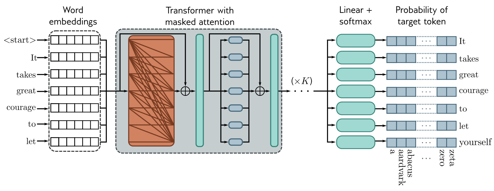
Generating text
To generate, an input sequence — possibly just the special <start> token — is fed into the network, which outputs probabilities over possible subsequent tokens. Either the most likely token is picked or one is sampled from the distribution. The extended sequence is fed back in to yield the distribution over the next token. Because prior embeddings do not depend on subsequent ones under masked self-attention, much of the earlier computation can be recycled.
- Beam search keeps track of multiple possible sentence completions to find the overall most likely sequence of words, which is not necessarily found by greedily choosing the most likely word at each step.
- Top-k sampling randomly draws the next word from only the top-\(K\) most likely possibilities, to prevent the system from choosing from the long tail of low-probability tokens and leading to an unnecessary linguistic dead end.
Scale and few-shot learning
In GPT3 the sequence lengths are 2048 tokens long and the total batch size is 3.2 million tokens. There are 96 transformer layers, some of which implement a sparse version of attention, each processing a word embedding of size 12288. There are 96 heads in the self-attention layers, and the value, query and key dimension is 128. It is trained with 300 billion tokens and contains 175 billion parameters.
A model on this scale can perform many tasks without fine-tuning. Given several examples of correct question and answer pairs and then another question, it often answers the final question correctly by completing the sequence — for instance, correcting English grammar from paired Poor English input and Good English output examples. It is argued on this basis that enormous language models are few-shot learners. However, performance is erratic in practice, and the extent to which the model is extrapolating from learned examples rather than interpolating or copying verbatim is unclear.
Learning outcomes
- contrast-transformer-paradigms Distinguish encoder, decoder and encoder-decoder transformers by their attention masking and their training objective.
Concepts
- masked-self-attention dot products for later positions are set to negative infinity before the softmax, so the whole sequence loss is computed in one forward pass without a position seeing its own answer
- dot-product-self-attention the mask is applied inside the same query-key dot-product computation, and nothing else in the layer changes
Encoder-decoder models: machine translation
Translation between languages is an example of a sequence-to-sequence task. One common approach uses both an encoder, to compute a good representation of the source sentence, and a decoder, to generate the sentence in the target language. This is aptly called an encoder-decoder model.
Consider translating from English to French. The encoder receives the sentence in English and processes it through a series of transformer layers to create an output representation for each token. During training, the decoder receives the ground truth translation in French and passes it through a series of transformer layers that use masked self-attention and predict the following word at each position. The decoder layers also attend to the output of the encoder. Consequently, each French output word is conditioned on the previous output words and the source English sentence.
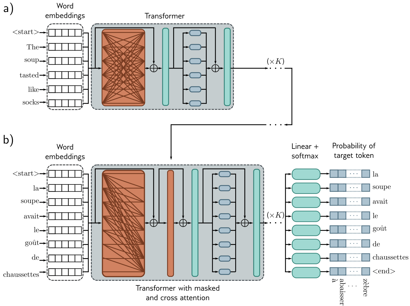
This is achieved by modifying the transformer layers in the decoder. Originally these consisted of a masked self-attention layer followed by a neural network applied individually to each embedding. A new self-attention layer is added between these two components, in which the decoder embeddings attend to the encoder embeddings. This uses a version of self-attention known as encoder-decoder attention or cross-attention, where the queries are computed from the decoder embeddings and the keys and values from the encoder embeddings.
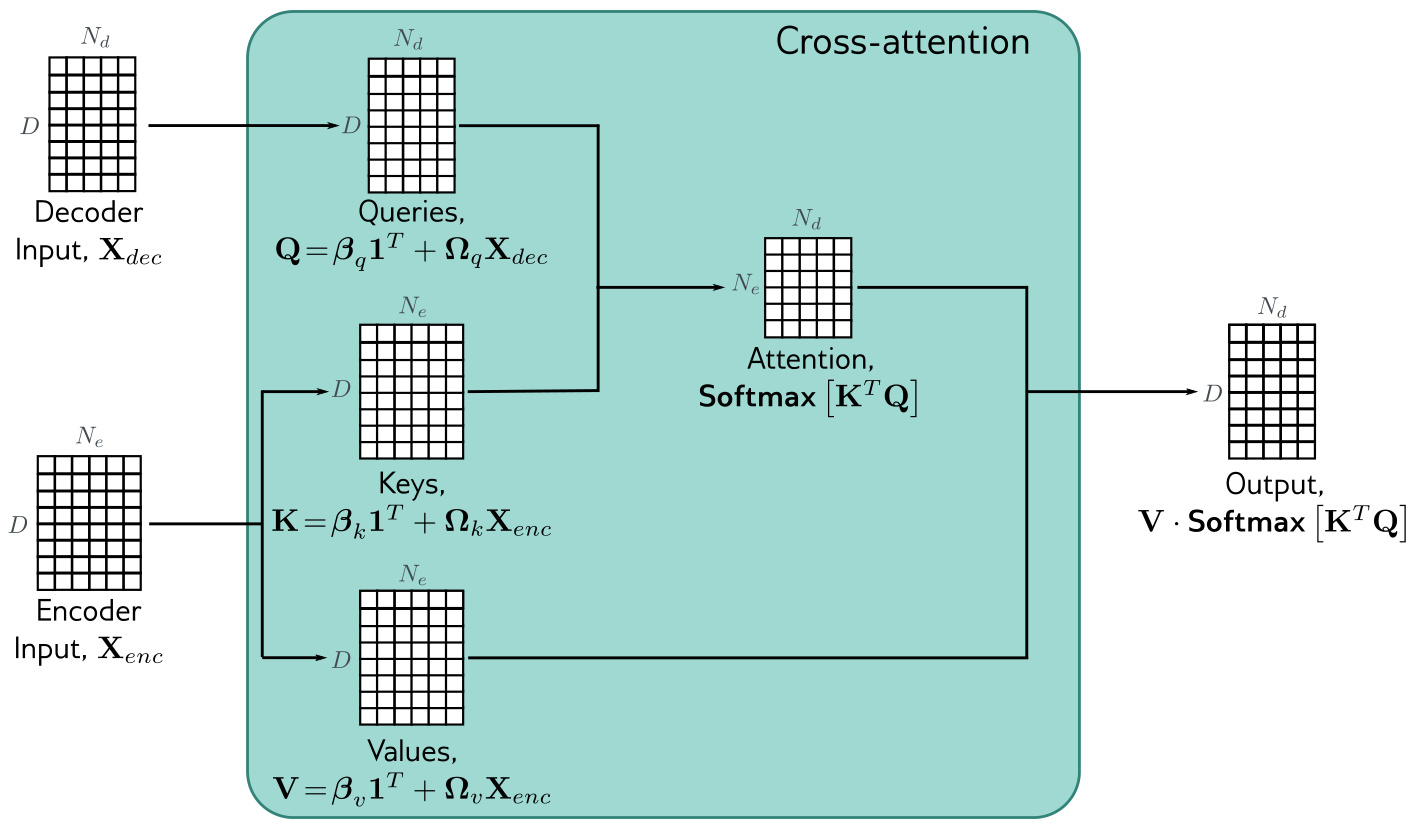
The arithmetic is unchanged from the scaled dot-product form. Writing \(N_d\) for the length of the decoder sequence and \(N_e\) for the length of the encoder sequence,
\[\mathbf{Q} = \boldsymbol\beta_q\mathbf{1}^T + \boldsymbol\Omega_q\mathbf{X}_{dec}, \quad \mathbf{K} = \boldsymbol\beta_k\mathbf{1}^T + \boldsymbol\Omega_k\mathbf{X}_{enc}, \quad \mathbf{V} = \boldsymbol\beta_v\mathbf{1}^T + \boldsymbol\Omega_v\mathbf{X}_{enc}\]
and the output \(\mathbf{V} \cdot \mathbf{Softmax}[\mathbf{K}^T\mathbf{Q}]\) has \(N_d\) columns, one per decoder position. For translation, the encoder contains information about the source language statistics and the decoder about the target language statistics.
The three paradigms are now complete, and a transformer model is classified by two questions: whether its self-attention is masked, and where its keys and values come from.
| Model | Self-attention | Keys and values | Trained by |
|---|---|---|---|
| Encoder | Unmasked | Own embeddings | Predicting masked tokens |
| Decoder | Masked | Own embeddings | Predicting the next token |
| Encoder-decoder | Masked in the decoder | Encoder output, in the cross-attention layer | Predicting the next output token |
Learning outcomes
- contrast-transformer-paradigms Distinguish encoder, decoder and encoder-decoder transformers by their attention masking and their training objective.
Scaling to long sequences
Since each token in a transformer encoder model interacts with every other token, the computational complexity scales quadratically with the length of the sequence. For a decoder model, each token only interacts with previous tokens, so there are roughly half the number of interactions, but the complexity still scales quadratically. These relationships are visualized as interaction matrices.
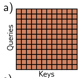
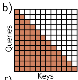
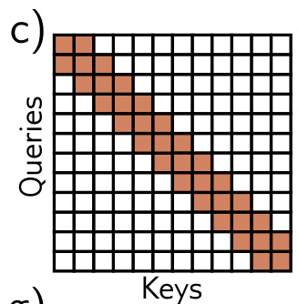
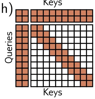
The quadratic increase in the amount of computation ultimately limits the length of sequences that can be used. Three lines of work address it: the first decreases the size of the attention matrix, the second makes the attention sparse, and the third modifies the attention mechanism to make it more efficient.
Decreasing the size of the attention matrix. Memory-compressed attention applies strided convolution to the keys and values, which reduces the number of positions in a way similar to downsampling in a convolutional network; attention is then applied between weighted combinations of neighbouring positions, where the weights are learned. The LinFormer was developed from the observation that the quantities in the attention mechanism are often low rank in practice, and projects the keys and values onto a smaller subspace before computing the attention matrix.
Making the attention sparse. Pruning the interactions is equivalently sparsifying the interaction matrix. In local attention, neighbouring blocks of tokens only attend to one another, which creates a block diagonal interaction matrix; information cannot pass from block to block, so such layers are typically alternated with full attention. GPT3 uses a convolutional interaction matrix alternated with full attention. Dilated patterns widen the receptive field across layers, as convolution kernels do in images. The extended transformer construction uses a set of global embeddings that interact with every other token; like the
<cls>token, these do not represent any word but serve to provide long-distance connections. BigBird combines global embeddings with a convolutional structure and a random sampling of possible connections.Modifying the mechanism. The terms in the numerator and denominator of the softmax operation have the form \(\exp[\mathbf{k}^T\mathbf{q}]\). This can be treated as a kernel function and expressed as the dot product \(\mathbf{g}[\mathbf{k}]^T\mathbf{g}[\mathbf{q}]\), where \(\mathbf{g}[\bullet]\) is a nonlinear transformation. That formulation decouples the queries and keys, so the matrix products can be reassociated and the attention computation made more efficient. To replicate the exponential exactly, \(\mathbf{g}[\bullet]\) must map its inputs to an infinite space. The linear transformer replaces the exponential term with a different similarity measure; the Performer approximates the infinite mapping with a finite-dimensional one.
The global-token and dilated patterns do not remove the all-pairs interaction so much as route it through intermediaries and across layers. A pure convolutional approach requires many layers to integrate information over large distances, which is why the sparse patterns are alternated with full attention rather than used alone.
Learning outcomes
- analyze-attention-complexity Analyse the quadratic cost of full self-attention and describe the main strategies that reduce it.
Transformers for images
Transformers were initially developed for text data, and applying them to images was not obviously promising for two reasons. First, there are many more pixels in an image than words in a sentence, so the quadratic complexity of self-attention poses a practical bottleneck. Second, convolutional nets have a good inductive bias because each layer is equivariant to spatial translation, and takes into account the 2D structure of the image; in a transformer network this must be learned. Transformer networks for images have nonetheless eclipsed the performance of convolutional networks for image classification, partly because of the enormous scale at which they can be constructed and the large amounts of data that can be used to pre-train them.
ImageGPT
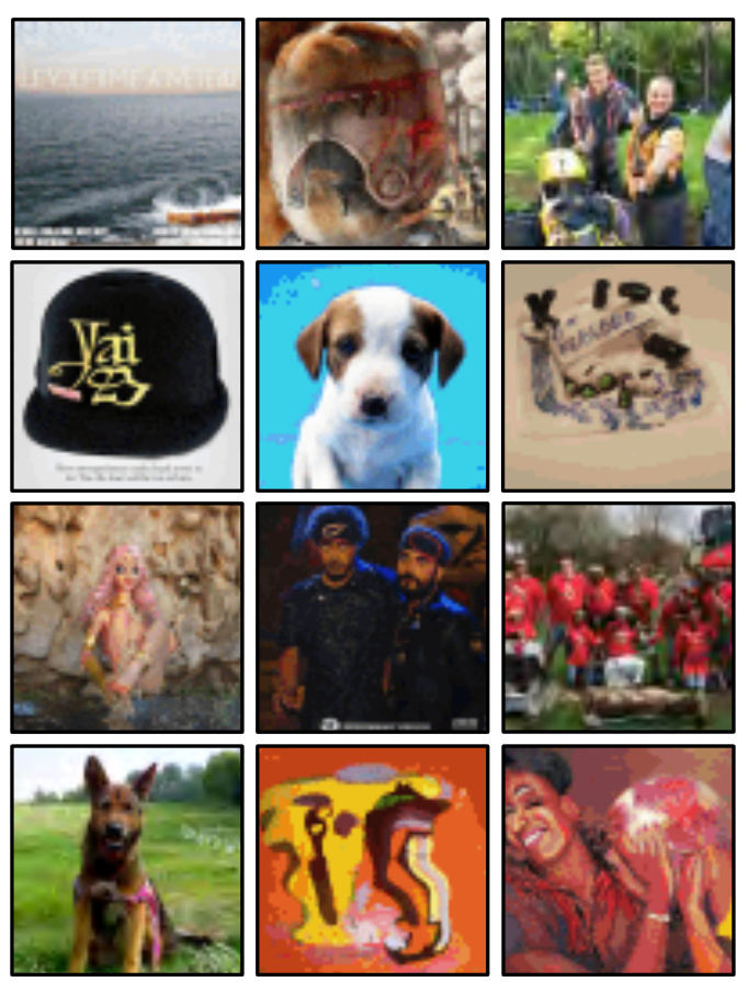
ImageGPT is a transformer decoder that builds an autoregressive model of image pixels: it ingests a partial image and predicts the subsequent pixel value. The quadratic complexity means that the largest model, which contained 6.8 billion parameters, could still only operate on \(64 \times 64\) images. To make this tractable, the original 24-bit RGB color space had to be quantized into a nine-bit color space, so the system ingests and predicts one of 512 possible tokens at each position. Images are naturally 2D objects, but ImageGPT simply learns a different positional encoding at each pixel; it must therefore learn that each pixel has a close relationship with its preceding neighbors and also with nearby pixels in the row above.
The internal representation of this decoder was used as a basis for image classification. Each pixel’s final embedding is averaged, and a linear layer maps these values to activations passed through a softmax. Pre-trained on a large corpus of web images and fine-tuned on the ImageNet database resized to \(48 \times 48\) pixels, with a loss combining a cross-entropy term for classification and a generative term for predicting the pixels, the system achieved a 27.4% top-1 error rate. This was worse than convolutional architectures of the time; it fails where the target object is small or thin.
Vision Transformer
The Vision Transformer tackled the problem of image resolution by dividing the image into \(16 \times 16\) patches. Each patch is mapped to an input embedding via a learned linear transformation, and these representations are fed into the transformer network. Standard 1D positional encodings are learned. It is an encoder model with a <cls> token, but unlike BERT it uses supervised pre-training on a large database of 303 million labeled images from 18,000 classes. The <cls> token is mapped via a final network layer to create activations fed into a softmax to generate class probabilities; after pre-training, the final layer is replaced with one that maps to the desired number of classes and the system is fine-tuned.
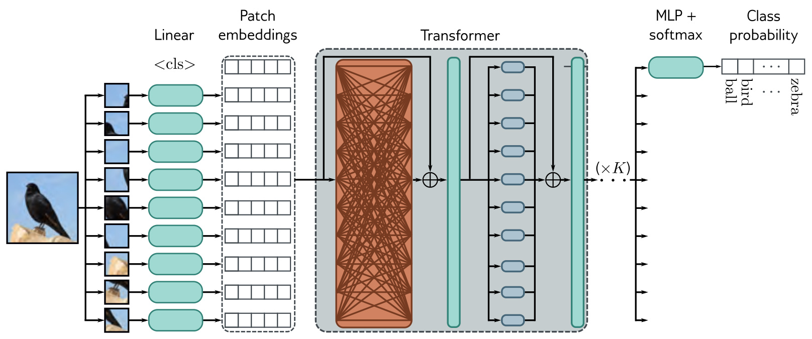
<cls> token is used to predict the class probabilities.For the ImageNet benchmark, this system achieved an 11.45% top-1 error rate. It did not perform as well as the best contemporary convolutional networks without supervised pre-training. The strong inductive bias of convolutional networks can only be superseded by employing extremely large amounts of training data.
Multi-scale vision transformers
The Vision Transformer operates on a single scale and has a receptive field that covers the whole image. Multi-scale models start with small high resolution patches and few channels, and gradually enlarge the receptive field, decrease the spatial resolution and increase the number of channels — as convolutional networks do.
The shifted-window or SWin transformer is an encoder transformer that divides the image into patches and groups these patches into a grid of windows within which self-attention is applied independently. These windows are shifted in adjacent transformers, so the effective receptive field at a given patch can expand beyond the window border. The scale is reduced periodically by concatenating features from non-overlapping \(2 \times 2\) patches and applying a linear transformation that maps these concatenated features to twice the original number of channels. This architecture has no <cls> token; it averages the output features at the last layer. The most sophisticated version of this architecture achieves a 9.89% top-1 error rate on the ImageNet database.
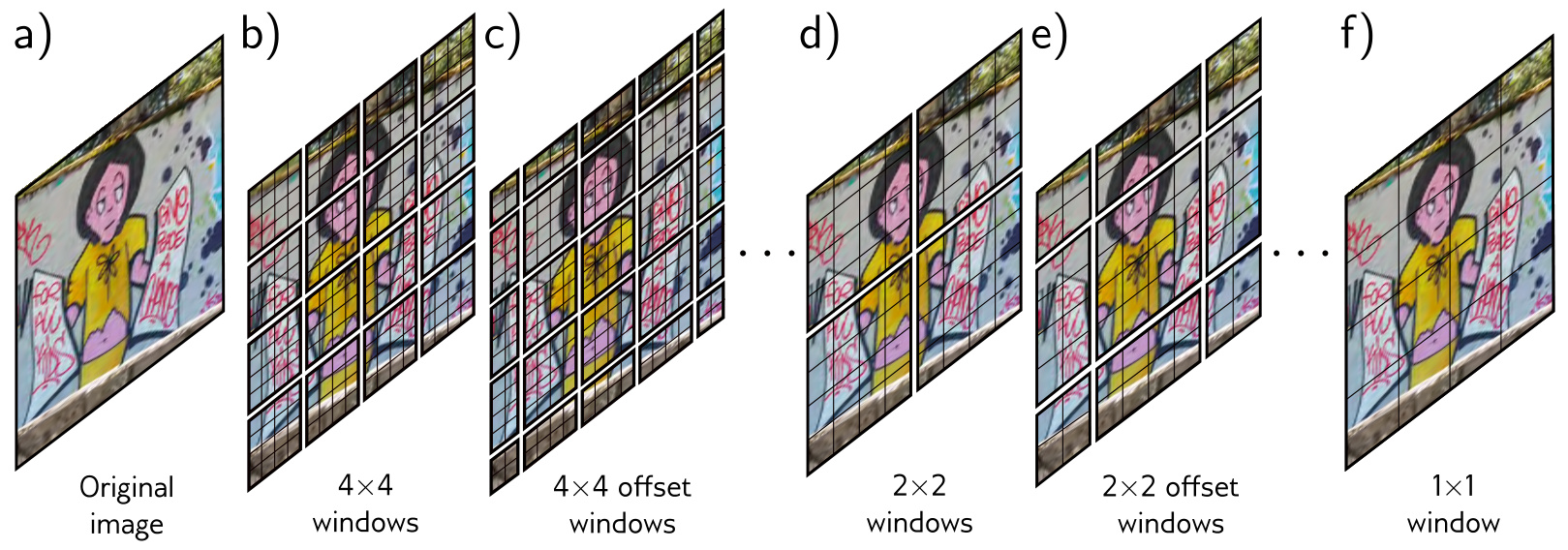
Dual attention vision transformers, or DaViT, alternate two types of transformers. In the first, image patches attend to one another and the self-attention computation uses all the channels. In the second, the channels attend to one another and the self-attention computation uses all the image patches. This architecture reaches a 9.60% top-1 error rate on ImageNet.
Learning outcomes
- adapt-transformers-to-images Describe how transformers are adapted to images by treating patches or pixels as tokens.
Concepts
- vision-transformer an encoder over \(16 \times 16\) patch tokens with a
<cls>token, which needs 303 million supervised pre-training images to reach an 11.45% top-1 error rate - positional-encoding the 2D layout of patches is supplied by learned 1D encodings, so the spatial structure is learned rather than built in
- multi-scale-vision-transformers attention within local windows, shifted in alternate layers, with \(2 \times 2\) patch merging between resolutions, restores the hierarchy convolutional networks have
- sparse-and-efficient-attention confining attention to a window is the same sparsification used for long text, applied here to make high-resolution images tractable
What this unit established
Self-attention dynamically routes information across variable-length sequences using learned, data-dependent query-key similarities.
Fixed-weight architectures cannot connect the word it to the word restaurant, because the connection depends on the words rather than on their positions.
Transformers divide into encoders, decoders and encoder-decoder models according to how attention is structured.
The mechanism is the same in all three; what differs is whether the attention matrix is masked and whether the keys and values come from the same sequence as the queries.
The quadratic cost of full self-attention is what limits the sequence length, and has produced sparse patterns, low-rank projections and kernel rewrites in response.
The \(N \times N\) attention matrix is the source of both the architecture’s strength, all-pairs interaction, and its cost.
Transformers adapt to vision by treating patches as tokens, surpassing convolutional networks when given massive datasets or hierarchical designs.
Nothing in self-attention is specific to text; what convolution supplies as an architectural bias, the transformer must obtain from data.
The next unit, 1 Understanding large language models, takes the decoder of this unit as the engine of a large language model and asks what scaling it produces: the two-stage lifecycle of self-supervised pretraining on unlabeled corpora followed by fine-tuning, the composition and compute cost of a pretraining corpus, and the zero- and few-shot in-context learning seen in GPT3 as a behaviour that emerges with scale rather than one trained for directly.
References
- Understanding Deep Learning, Simon Prince, 2026 — Link — Page 221-253