Lecture notes — I Foundations
ver. 1.0.0, i_foundations
ver. 1.0.0 · 2026-08-22 10:31:37
Where we are
This is the first unit of the Reinforcement Learning module, so we start from nothing. No previous unit of this module is assumed. What is assumed is the supervised setting you already know: a fixed dataset, a ground-truth label for every example, a loss, and a gradient step that reduces it.
In this module the data does not exist yet. The agent has to go out and generate it, and the only feedback it gets is a number.
In this unit we will:
- See why that single number makes reinforcement learning a different kind of problem from supervised learning.
- Build the vocabulary — states, actions, rewards, trajectories, policies, Markov decision processes — that every later derivation assumes.
- Map the landscape of algorithms by asking one question of each: what does it learn?
- Face the four challenges that make the field hard in practice, and finish with a complete worked case study.
We will not derive any algorithm here. The aim is that by the end you can state a control problem in reinforcement-learning terms and say which family of methods should attack it.
The single source for this unit is The Little Book of Reinforcement Learning, Alexandre Torres Leguet, 2026, chapters 1 and 2 together with the Practical Notes.
What you will be able to do
rl-vs-supervised— Explain how RL’s evaluative reward signal differs from a supervised label, and state the credit assignment problem it creates.interaction-loop— Write the agent-environment interaction loop and describe a trajectory in terms of states, actions and rewards.markov-and-mdp— Test whether an observation is Markov and formalise a task as an MDP with a policy \(\pi(A_t \mid S_t)\).training-loop-nonstationarity— Describe the collect-then-update training loop and explain why the agent’s own data distribution keeps shifting.core-challenges— Diagnose the four core RL challenges — credit assignment, optimisation instability, reward design and exploration versus exploitation — in a given task.algorithm-taxonomy— Classify an RL algorithm by which object it learns: a policy, a value function, or a model of the environment.choose-algorithm-family— Compare the common algorithm families and pick one for a task from its action space, sample cost and stability needs.design-an-rl-problem— Design a complete RL formulation for a concrete control task, including reward, curriculum and demonstration bootstrapping.
What we will cover
The source introduces the following concepts. Each is defined where it is first used.
- Reinforcement Learning — the study of agents that learn to act by trial and error, guided by scalar rewards rather than by direct supervision.
- Credit Assignment Problem — the difficulty of deciding which past actions deserve credit or blame for a reward observed later.
- Interaction Loop — the cycle in which the agent observes a state, acts, and the environment returns a next state and a reward.
- Markov Property — the assumption that the current state contains everything needed to predict how the environment evolves.
- Markov Decision Process (MDP) — the formal object \((\mathcal{S}, \mathcal{A}, p, r)\) underlying most of reinforcement learning.
- Policy — the decision rule \(\pi(A_t \mid S_t)\) that an RL algorithm ultimately learns.
- Training Loop — the alternation between collecting experience and updating the agent from it.
- Reward Hacking — an agent maximising a misspecified reward without solving the intended task.
- Exploration-Exploitation Dilemma — the trade-off between using what is already known to work and trying what might work better.
- Model-Free RL Methods — methods that learn a policy or a value function without an explicit predictive model of the environment.
- Model-Based RL Methods — methods that learn or are given a model of the environment in order to plan.
- Actor-Critic Methods — methods that learn a policy and a value function together.
- Curriculum Learning — training on a deliberately easier version of the problem first, then raising the difficulty.
Why a reward is not a label
We begin with the single distinction on which the whole field rests.
Reinforcement Learning (RL) is the study of agents that learn to act by trial and error: they interact with an environment, receive rewards, and adjust their behaviour accordingly.
That definition invites an objection, and the source raises it immediately. Training a convolutional network to classify images from CIFAR-10 is also a decision problem. The model learns, during training, to decide how to classify a given image, and a learning signal tells it how well it is doing. How is that different from a model learning to play Breakout, which updates its weights based on the game score? In both cases the goal of training is to optimise some metric.
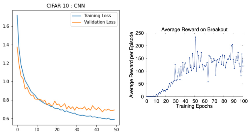
The difference is in the nature of the signal.
When classifying an image, the signal is the ground-truth label for that image. It is a direct target: it tells the model exactly what its output should have been.
Optimising against that signal is enough to learn to classify the image correctly. The correction is handed to you.
When an agent plays a move in Breakout, the signal is the game score. That score does not depend only on the action just taken.
A good action may lead to a bad immediate score, and a bad action may lead to a good one. The reward is not a direct target, because it never says which action should have been played.
This is the core difficulty of RL, and it has a name. The credit assignment problem is the agent’s task of figuring out which of its past actions deserve credit — or blame — for the rewards it eventually observes.
The vocabulary the source uses is worth fixing now. An RL problem involves an agent interacting with an environment, taking actions and receiving rewards as a consequence. An RL algorithm provides a recipe to update the agent based on those rewards, so that it performs better in the future. In doing so, the algorithm tries to solve the credit assignment problem: it must determine which actions were responsible for the positive or negative rewards received, and reinforce or discourage them accordingly.
The two figures above differ in more than their axes. The CIFAR-10 loss falls smoothly and settles. The Breakout reward climbs, but it jitters violently from epoch to epoch. That difference is not noise in the plotting; it is the shape of the problem, and we will return to it twice more in this unit.
Ask what your training signal tells you. If it names the correct output for each input, you have a supervised problem, whatever else is going on. If it only scores an outcome that several of your decisions jointly produced, you have an RL problem and a credit assignment problem with it.
Learning outcomes
- rl-vs-supervised Explain how RL’s evaluative reward signal differs from a supervised label, and state the credit assignment problem it creates.
Concepts
- reinforcement-learning defines RL as agents learning via trial and error, and contrasts its reward signals with supervised ground-truth targets
- credit-assignment-problem explains why credit assignment is the core challenge distinguishing RL from supervised learning
The interaction loop
The interaction between the agent and the environment is at the core of RL. It is worth defining precisely, because the notation fixed here is used for the rest of the module.
At each time step \(t\):
- The agent observes the current situation of the environment, called the state, denoted \(S_t\). This is what the agent knows about the situation.
- Based on this state, it chooses an action \(A_t\). This is what the agent decides to do.
- Once the action is taken, the environment reacts. It transitions to a new state \(S_{t+1}\) and returns a reward \(R_{t+1}\), the feedback signal received after taking action \(A_t\) in state \(S_t\).
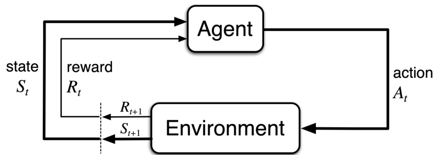
Repeating this produces a sequence called a trajectory:
\[S_0, A_0, R_1, S_1, A_1, R_2, S_2, A_2, R_3, \dots\]
When this trajectory reaches a terminal state, it is also called an episode. In a game, an episode may correspond to one full game; in robotics, to one trial. In continuing tasks, the interaction may continue without a clear end.
Framing concrete tasks
These definitions are abstract on purpose. In particular the reward can be \(0\) most of the time, except at the end of the episode. Framing the loop correctly is most of the work in applying RL, so it is worth walking the source’s four examples.
Breakout. State: the current game screen, or features extracted from it — ball position, paddle position, brick layout. Action: move left, move right, or stay still. Reward: positive when hitting bricks or winning, negative when losing the ball.
Cart balancing. State: cart position, cart velocity, pole angle, and pole angular velocity. Action: push the cart left or right. Reward: \(+1\) for every time step the pole remains balanced.
Robot navigation. State: robot position, distance to obstacles, and direction of the goal. Action: move forward, turn left, turn right, or stop. Reward: positive for reaching the goal, negative for collisions, and a small penalty for taking too long.
Recommender system. State: information about the current user, such as past clicks, watch history, or preferences. Action: recommend one item among many possible choices. Reward: positive if the user clicks, watches, or buys; little or no reward otherwise.
Notice how much design sits inside each of these. Cart balancing gets a reward at every step; the recommender gets one only when the user acts. Robot navigation adds a time penalty that nothing in the physical task demanded. These are decisions, not facts, and section five returns to their consequences.
Key ideas
- One time step is: observe \(S_t\), choose \(A_t\), receive \(R_{t+1}\) and \(S_{t+1}\).
- A trajectory is the whole sequence; an episode is a trajectory that reaches a terminal state.
- State, action and reward are abstract slots. Filling them for a given task is the modelling work.
Learning outcomes
- interaction-loop Write the agent-environment interaction loop and describe a trajectory in terms of states, actions and rewards.
Concepts
- interaction-loop breaks the agent-environment cycle down into states, actions, rewards, trajectories and episodes
- credit-assignment-problem notes that the RL algorithm’s update must decide how credit and blame are spread across the interactions
The Markov property and MDPs
The definition of the interaction loop is universal. It imposes no limitation on the environments we may consider. To make the problem tractable, however, we usually assume one extra property of the environment: the Markov property.
It says that the current state \(S_t\) contains all the information needed to predict the evolution of the environment. No additional information from the past — earlier states, for instance — is needed to predict what comes next. As the state fully describes the environment, the agent has all the information it needs to make a guess about the future and choose its action accordingly.
It does not state that the future is determined by \(S_t\). The next state and reward may still be random. It says only that whatever randomness there is depends on \(S_t\) alone, not on the full history.
When an observation is not Markov
Whether an environment is Markovian depends on how we define the state. Breakout is the source’s example.
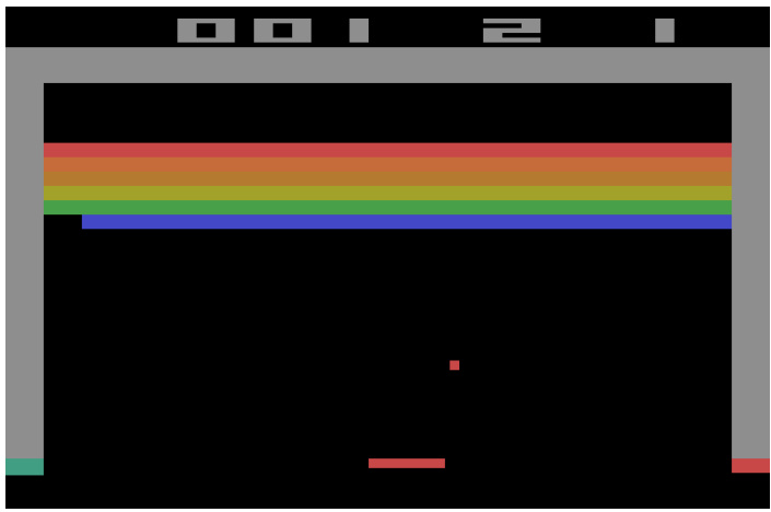
A single frame is not enough to tell where the ball is heading, but a stack of a few additional past frames is. The single-frame formulation therefore violates the Markov property, since adding past information should not be necessary to predict the future.
The common fix is to modify the definition of the state. Instead of a single frame, use a stack of the last \(4\) frames, which taken together give information about the ball velocity and thus its future trajectory. In fact one can always make an environment Markovian by including enough history in the state, although the result may not be tractable.
This is why we sometimes distinguish the state — the true, fully descriptive state of the environment — from the observation, the part of the state the agent has access to. Often we say “state” and mean “observation”, because we assume the environment, as we define it, is Markovian.
The MDP and the policy
The framework just described — a set of states \(\mathcal{S}\), a set of actions \(\mathcal{A}\), a transition function \(p(s' \mid s, a)\) and a reward function \(r(s, a)\) that model the environment dynamics — is formally called a Markov Decision Process (MDP). It is the mathematical object underlying most of RL.
The assumption has a direct consequence for the agent. Since \(S_t\) contains everything needed to predict the future, an optimal decision rule needs only depend on \(S_t\). That decision rule is called the policy:
\[\pi(A_t \mid S_t).\]
The policy is what the RL algorithm ultimately learns. Note what the Markov property has bought us: the policy carries no memory. It is a function of the current state, and the whole history before \(t\) can be discarded.
Learning outcomes
- markov-and-mdp Test whether an observation is Markov and formalise a task as an MDP with a policy \(\pi(A_t \mid S_t)\).
- interaction-loop Write the agent-environment interaction loop and describe a trajectory in terms of states, actions and rewards.
Concepts
- markov-property defines the Markov property and the techniques, such as frame stacking, that make an observation satisfy it
- markov-decision-process introduces the formal MDP framework of states, actions, transition dynamics and reward function
- policy defines the policy \(\pi(A_t \mid S_t)\) as the primary object an RL algorithm learns
The training loop
The interaction loop explains how the agent interacts with the environment and generates experience. The training loop explains how the agent improves from this experience.
A typical training loop looks like this:
- The agent interacts with the environment.
- It collects states, actions and rewards.
- It uses this experience to update its policy.
- It interacts again using its new policy.
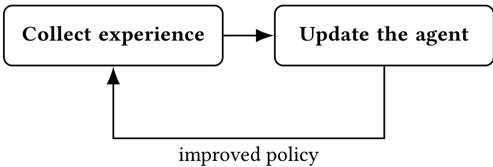
Depending on the method, the update step may try to increase the probability of actions that led to good outcomes, estimate how good a state or an action is, learn a model of the environment to better predict it, or combine several of these ideas. The next four sections are exactly that list.
Why this is not supervised learning with extra steps
So far the description sounds familiar. We take a batch of data and use it to update a model, inside a loop that runs until we are satisfied with performance. The update rule may differ from the supervised one, but is the overall picture not the same?
In a way, yes. But there is one point that makes RL much more subtle.
The data collected by the agent depends on the policy currently being followed. As the policy changes, the data distribution changes as well. A poor update can therefore lead the agent to visit very different states, collect worse experience, and receive fewer rewards, making learning collapse.

In supervised learning the data distribution is fixed. A bad update may hurt performance, but the model still learns from the same dataset, and the target it is trying to fit does not depend on its own predictions. That is the assumption the supervised training loop makes and RL cannot.
Interaction loop: how the agent and the environment produce experience.
Training loop: how this experience is used to improve the agent.
Learning outcomes
- training-loop-nonstationarity Describe the collect-then-update training loop and explain why the agent’s own data distribution keeps shifting.
- rl-vs-supervised Explain how RL’s evaluative reward signal differs from a supervised label, and state the credit assignment problem it creates.
Concepts
- training-loop details the four-step training cycle and explains how a changing policy alters the data distribution
- policy shows how updating the policy in turn determines what data is collected next
- interaction-loop contrasts generating experience in the environment with improving the agent from it
The four core challenges
We now name the four recurring difficulties. This section is the diagnostic toolkit for the rest of the module: when a later algorithm looks complicated, ask which of these four it was built to attack.
Credit assignment problem. A reward obtained at timestep \(100\) does not necessarily depend on the action taken at timestep \(99\). It may instead depend on an action taken much earlier, for example at timestep \(50\).
This makes it difficult to determine which actions should be reinforced.
Optimisation instability. In RL the agent generates its own training data. As the policy changes, the data distribution changes as well.
A poor update may lead the agent to collect worse trajectories, which in turn makes future learning harder. This is why many popular algorithms, such as Trust Region Policy Optimization (TRPO) or Proximal Policy Optimization (PPO), are built around the idea of taking careful policy updates.
Reward function. Designing a good reward function is often one of the hardest parts of applying RL to a new problem.
If the reward is too sparse — for example given only at the end of the episode — a randomly initialised agent may never observe any useful signal. If it is too dense or poorly specified, the agent may learn to maximise the reward in a way that does not actually solve the intended task. This phenomenon is called reward hacking.
Exploration-exploitation dilemma. The agent must choose between exploiting actions that already seem promising and exploring new actions that may lead to better outcomes.
The trade-off is difficult because exploration may be costly in the short term, yet necessary to discover good strategies.
The last of the four has a further wrinkle worth stating separately. During training, we want enough exploration to discover good strategies, but also enough exploitation to actually get a learning signal. During evaluation, we want to maximise exploitation to achieve the best performance. The balance is therefore not a single constant; it is a schedule.
Note also how the first two are linked to what we have already built. Credit assignment is the consequence of an evaluative reward, from section one. Optimisation instability is the consequence of the shifting data distribution, from section four. Reward design and exploration are new, and both are decisions the engineer makes rather than properties of the environment.
Learning outcomes
- core-challenges Diagnose the four core RL challenges — credit assignment, optimisation instability, reward design and exploration versus exploitation — in a given task.
- training-loop-nonstationarity Describe the collect-then-update training loop and explain why the agent’s own data distribution keeps shifting.
Concepts
- credit-assignment-problem details how rewards at distant timesteps complicate attribution to earlier actions
- reward-hacking warns against dense rewards that an agent can maximise without solving the target task
- exploration-exploitation-dilemma explains the tension between trying new actions and using known good ones, in training and in evaluation
Learning a policy
We now turn to the taxonomy of RL algorithms. The organising question is a single one: what object does the algorithm try to learn during the training loop? Algorithms differ by their answer, and knowing which object a method learns is, in the source’s words, one of the first reflexes to have when stumbling upon a new algorithm.
The most direct answer is the first we take. One of the objects an RL algorithm may learn is the policy itself, often denoted \(\pi\). It directly tries to learn which action to take. We usually talk about policy-based methods, or policy optimization.
The update step of such a method reads:
Given the previous batch of experience, update the policy to make it choose actions that lead to higher rewards.
That is the whole idea. There is no intermediate quantity. The experience says which actions were followed by higher rewards, and the parameters move so that those actions become more probable.
The alternative: deriving the policy
If we are not directly learning a policy, we derive it from another object that we learn. That object usually conveys some kind of prediction about the future of the environment. Being in a given state, querying this object gives us information about the different possible futures, allowing us to choose the best action. We derive the policy on the fly, without explicitly learning it.
There are two such objects, and they give the next two sections:
- A model of the environment, which predicts how the environment evolves.
- A value function, which estimates how good a state or an action is.
The two policy-based algorithms to keep in mind are REINFORCE and Group Relative Policy Optimization (GRPO). Both are model-free: they do not build any explicit predictor of the environment. The next unit derives their gradients.
These objects are not exclusive. An algorithm may try to learn several of them at the same time, and the most widely used methods do exactly that. We reach those combinations in two sections’ time.
Learning outcomes
- algorithm-taxonomy Classify an RL algorithm by which object it learns: a policy, a value function, or a model of the environment.
Concepts
- policy introduces policy-based algorithms that parameterise and update \(\pi\) directly to favour high-reward actions
Learning values
The second branch stores no policy at all. It stores an estimate of how good things are, and lets the policy fall out of the estimate.
The object here is a value function, often denoted \(V\) or \(Q\). The goal of such a function is to estimate how good a state is, or how good it is to take a given action in a given state, based on the rewards that are expected to be received in the future.
The update step reads:
Given the previous batch of experience, update the value function to better estimate the value of the states and actions.
Two forms appear throughout the module.
\(V(s)\) estimates how good state \(s\) is.
It scores a situation, not a decision. On its own it does not tell you which action to take from \(s\).
\(Q(s, a)\), the action-value function, estimates how good it is to take action \(a\) in state \(s\).
This is the form value-based methods most often learn, precisely because a decision falls straight out of it.
Given \(Q\), the policy is then derived implicitly and on the fly by choosing the action with the highest estimated value. Nothing is stored beyond the value estimates.
What this buys and what it costs
Notice the relationship to the challenges of the previous section. A value function estimates the rewards expected in the future from a given state or action. It therefore converts a reward that arrives at the end of an episode into a per-state quantity that can be consulted at any step. That is a direct line of attack on credit assignment, and it is why the next unit spends most of its length on this branch.
The cost is visible in the greedy step. Choosing the action with the highest estimated value requires a maximisation over the action set. That maximisation is immediate when the actions are few and discrete, and considerably less so otherwise. Deep Q-Network (DQN) is the canonical value-based, model-free algorithm, and it is an Atari agent with a handful of joystick actions.
Learning outcomes
- algorithm-taxonomy Classify an RL algorithm by which object it learns: a policy, a value function, or a model of the environment.
- core-challenges Diagnose the four core RL challenges — credit assignment, optimisation instability, reward design and exploration versus exploitation — in a given task.
Concepts
- model-free-methods introduces value estimation, through \(V\) or \(Q\), as the model-free alternative to learning a policy directly
Learning a model
The third option is to learn the environment itself.
One form the learned object can take is a model of the environment. This model is trained to predict how the environment evolves — typically its next state and reward — from the current state and action. That the current state and action suffice is exactly the Markov property, put to work: it is what licenses a predictor of the form \(p(s', r \mid s, a)\) with no history argument.
This is called a model-based approach. The update step reads:
Given the previous batch of experience, update the environment model to better predict the future.
Read that carefully. The direct goal here is not to maximise rewards, but to better predict the environment. Once such a model has been learned, it can then be used to derive or improve a policy.
Planning
The main advantage is that a model allows planning. Instead of acting immediately, the agent can use the model to imagine possible futures and choose actions more carefully. The deliberation happens inside the learned simulator, where a rollout costs nothing but computation, rather than in the real environment, where it costs a trial.
Model-based methods learn, or are sometimes given, this model. Probabilistic Ensembles with Trajectory Sampling (PETS) and AlphaGo Zero are the source’s two examples. AlphaGo Zero is the case where the model is given rather than learned: the rules of Go define the transitions exactly.
The contrast
By contrast, model-free methods do not try to explicitly learn a model of the environment. These algorithms may still capture some model of the environment implicitly, but they do not learn an explicit predictive model that can be used to simulate or predict future states and rewards. Both branches of the previous two sections — policy-based and value-based — are model-free in this sense.
Learning outcomes
- algorithm-taxonomy Classify an RL algorithm by which object it learns: a policy, a value function, or a model of the environment.
Concepts
- model-based-methods introduces learning a predictive model of transitions and rewards in order to plan
- model-free-methods defines model-free methods as those that build no explicit predictive model of the environment
- markov-property justifies modelling the next state and reward from the pair \((s, a)\) alone
Common combinations and choosing a family
The three objects each have a different nature, and each tries to predict a different aspect of the environment. An RL algorithm may try to learn several of them at the same time. Rather than enumerating all combinations, we follow the source and focus on the patterns that appear most often in practice.
Value-based, model-free. Learn a value function, most often \(Q(s, a)\). The policy is derived implicitly by choosing the action with the highest estimated value.
Example: Deep Q-Network (DQN).
Policy-based, model-free. Learn the policy directly, increasing the probability of actions that led to higher rewards in the past.
Examples: REINFORCE, Group Relative Policy Optimization (GRPO).
Actor-critic, model-free. Learn a policy, called the actor, and a value function, called the critic. The actor chooses actions; the critic evaluates how good states or actions are, and helps guide and stabilise the learning of the actor.
Examples: Trust Region Policy Optimization (TRPO), Proximal Policy Optimization (PPO). This combination is extremely common in modern RL, because it often provides a good compromise between performance and stability.
Model-based. Learn, or be given, a model of the environment, and plan with it.
Examples: PETS, AlphaGo Zero.
Hybrid. Combine several of the previous ideas at once — a policy, a value function, and a model of the environment, simultaneously.
Examples: MuZero, Dreamer.
Choosing a category
The source gives two criteria for a given problem.
The environment. Is it natural or easy to model? If so, model-based methods can be effective. Is it easier to estimate values, or to directly learn a policy?
The amount of data available. If data is limited, use an algorithm that is able to re-use past experience.
Both criteria are about the problem, not about the algorithm’s reputation. The first asks whether the dynamics are something you can write down or learn cheaply — the rules of a board game, yes; contact-rich manipulation, considerably less so. The second is a question about cost: each interaction with a real robot or a paying user is expensive, and a method that discards a batch after one update will need many more of them.
Key ideas
- Model-free splits three ways: value-based, policy-based, and actor-critic which learns both.
- Model-based splits two ways: planning with a model, and hybrid methods that add a policy and/or a value function.
- Actor-critic is the common modern default because it trades performance against stability well.
- Choose on the environment’s modelability and on how much data you can afford to collect.
Learning outcomes
- choose-algorithm-family Compare the common algorithm families and pick one for a task from its action space, sample cost and stability needs.
- algorithm-taxonomy Classify an RL algorithm by which object it learns: a policy, a value function, or a model of the environment.
Concepts
- model-free-methods surveys the value-based, policy-based and actor-critic variants of model-free RL
- actor-critic-methods details how an actor chooses actions while a critic evaluates them and stabilises learning
- model-based-methods examines model-based planning and the hybrid architectures built on top of it
Case study: landing a Starship
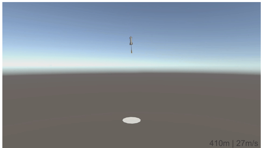
We close by carrying one task end to end. The goal of the project is to control the final phase of descent of a Starship rocket and make the vehicle land upright on a landing pad.
Formulating the MDP
The environment was built in Unity, and training was done with the Unity ML-Agents toolkit, using PPO — a model-free, actor-critic RL algorithm.
- State. The physical situation of the rocket at a given time: where it is, how fast it moves, and how it is oriented. It is a vector containing \(11\) real-valued numbers.
- Action. The control decisions available to the agent: firing the engines, changing their direction, or using side thrusters. The agent must choose among \(162\) discrete actions combining engine on/off, engine gimballing, and RCS commands.
- Reward. Meant to capture the objective of the task: a successful landing.
This is a natural RL problem because it is easy to frame as a game. In other words, we do not tell the agent how to land. We only define what counts as success, and let it discover a strategy through trial and error.
The four challenges, in the field
Credit assignment. Trajectories typically span thousands of time steps, and the reward is only given at the end of the episode. A successful landing may depend on a sequence of thousands of actions, and it is not clear which ones were responsible.
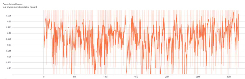
Optimisation instability. The reward curve below is the only signal available during training to tell whether the agent is improving. It is very different from a smooth supervised loss curve.
Reward function. This was the most difficult part of the project, and it is worth following in full.
Exploration-exploitation. During training, PPO ensures that the policy always has a bit of randomness, which allows for some exploration — trying actions which are, according to the agent’s knowledge, suboptimal.
Designing the reward
Ideally we want a simple reward function that directly encodes the real goal: \(+1\) whenever the landing is successful, and \(0\) otherwise. But this reward is extremely sparse. At the beginning of training, landing a rocket is almost impossible for a random policy, which starts \(5000\)m in the air with a random orientation. Even given an enormous exploration budget, obtaining a single successful landing by chance is extremely unlikely, so the agent never receives any learning signal.
One solution is a denser reward: a small positive reward for getting closer to the landing pad, a small negative reward for having too high a velocity. But this is very delicate, as it is prone to reward hacking. The agent may learn to hover at a certain height above the landing pad, which gives a good reward for being close, but never actually land.
The solution adopted was curriculum learning: instead of starting from the full problem, start with an easier version of it, so that random exploration actually leads to some successful landings. The rocket was spawned much closer to the ground, or with a more favourable orientation. The agent can then experience success more easily, and gradually learn to handle more difficult situations.
The sparse reward function was finally chosen in combination with curriculum learning. Even that was not enough at the beginning of training, so imitation learning was also used briefly, providing demonstrations of successful behaviour so that the agent could experience reward at least a few times. Once it had discovered trajectories leading to success, standard RL took over. The imitation phase accounted for less than \(0.001\%\) of the total training. All the real progress came from RL on harder and harder trajectories, spawning the spaceship from \(500\)m at the beginning of the curriculum to \(5000\)m in the sky with random orientation at the hardest level.
The curriculum explains the shape of the figure above. Landings were made harder and harder as training progressed, so a flat or falling reward can mean the task got harder rather than the agent got worse. Randomness in the policy matters here for the same reason: because the setup changes during training, the agent must keep exploring and not get stuck in a local optimum that only works for the current curriculum level.
The project is documented at github.com/alxndrTL/Landing-Starships. The book’s companion repository, github.com/alxndrTL/little-book-rl, holds one-file Python and PyTorch implementations of every algorithm, supplementary material for proofs, and notebooks to reproduce all figures.
Learning outcomes
- design-an-rl-problem Design a complete RL formulation for a concrete control task, including reward, curriculum and demonstration bootstrapping.
- core-challenges Diagnose the four core RL challenges — credit assignment, optimisation instability, reward design and exploration versus exploitation — in a given task.
- choose-algorithm-family Compare the common algorithm families and pick one for a task from its action space, sample cost and stability needs.
Concepts
- actor-critic-methods illustrates PPO, an actor-critic algorithm, driving the rocket landing controller through Unity ML-Agents
- curriculum-learning shows how raising the spawn altitude from 500m to 5000m made an otherwise hopeless sparse reward learnable
- reward-hacking discusses how proximity-based shaping risks a hovering policy instead of a landing one
- credit-assignment-problem examines attribution across the thousands of timesteps preceding touchdown
- exploration-exploitation-dilemma explains why the policy must stay stochastic when the curriculum keeps changing the task
The vocabulary is now in place
You can now state a control problem in RL terms and say which family should attack it.
A reward is evaluative, not instructive. It scores the action taken and never names the action that should have been taken.
That single fact separates RL from supervised learning, and it produces the credit assignment problem: a reward at timestep 100 may be owed to an action at timestep 50.
The interaction loop is observe \(S_t\), act \(A_t\), receive \(R_{t+1}\) and \(S_{t+1}\); repeated, it produces a trajectory, and a trajectory reaching a terminal state is an episode.
State, action and reward are abstract slots. Filling them for Breakout, a cart, a robot or a recommender is the modelling work, and it is where most applied RL effort goes.
Under the Markov property, \(S_t\) contains everything needed to predict the future, and the task is a Markov Decision Process \((\mathcal{S}, \mathcal{A}, p, r)\).
The payoff is that the policy can be written \(\pi(A_t \mid S_t)\), with no memory. When an observation breaks the assumption, redefine the state — a stack of four Breakout frames carries the ball’s velocity.
The training loop alternates collecting experience with updating the agent, and the agent generates its own data.
Every policy update changes the data distribution. A bad update collects worse trajectories, which makes the next update worse still. The supervised assumption of a fixed dataset simply does not hold.
Four challenges recur: credit assignment, optimisation instability, reward design, and exploration versus exploitation.
A sparse reward gives a random agent nothing to learn from; a dense one invites reward hacking. Neither is safe by default, and the choice is yours to make.
Every algorithm is classified by what it learns: a policy, a value function, or a model — and the common methods learn more than one.
DQN learns values; REINFORCE and GRPO learn a policy; TRPO and PPO learn both; PETS and AlphaGo Zero plan with a model; MuZero and Dreamer combine all three.
A hard task is made learnable by changing the task, not only the algorithm.
The Starship agent learned from a sparse reward because curriculum learning raised the spawn altitude from 500m to 5000m, and because a brief imitation phase — under \(0.001\%\) of training — showed it success at least a few times.
II Diving Deeper turns this vocabulary into working algorithms. It defines \(V^\pi\) and \(Q^\pi\) and their Bellman equations, then places dynamic programming, Monte Carlo methods and temporal-difference learning on a single map of backup depth and width. It draws the on-policy/off-policy line with SARSA and Q-learning, scales Q-learning to raw pixels as a Deep Q-Network, derives the policy gradient and reduces its variance three times over, and ends at PPO’s clipped objective. Every one of those is an answer to a problem we have named here.
References
- The Little Book of Reinforcement Learning, Alexandre Torres Leguet, 2026 — Link — Page 10-39