Lecture notes — II Diving deeper
ver. 1.0.0, ii_diving_deeper
ver. 1.0.0 · 2026-08-22 10:33:25
From vocabulary to algorithms
I Foundations gave you the language of reinforcement learning: the interaction loop between agent and environment, the Markov property and the MDP that formalises it, the training loop with its shifting data distribution, the core challenges of the field, and a taxonomy of algorithms sorted by what they learn. What it did not give you was a single algorithm you could run.
This unit supplies them. We work through Chapters 3 and 4 of The Little Book of Reinforcement Learning, and we will find that the algorithms are far less varied than their names suggest.
- Value-based methods occupy the first half. We define value functions, then show that Dynamic Programming, Monte Carlo and Temporal-Difference learning are the same Bellman backup traversed differently. From there we reach SARSA, Q-learning, \(n\)-step returns, TD(\(\lambda\)) and Deep Q-Networks.
- Policy optimisation methods occupy the second. We derive the policy gradient, reduce its variance three times over, and end at PPO’s clipped trust region.
Two themes run through everything, and it is worth watching for both from the start.
The bias-variance trade-off in estimating returns.
Every method in this unit either accepts a noisy but honest estimate of the future, or a quieter estimate that is partly a guess. There is no third option.
The on-policy / off-policy distinction.
This decides whether you are allowed to reuse data your current policy did not collect, and therefore whether a replay buffer is available to you at all.
The source for this unit is The Little Book of Reinforcement Learning, Alexandre Torres Leguet, 2026, Chapters 3 and 4. Every algorithm shown here has a reference implementation in the companion repository little-book-rl.
What you will be able to do
value-functions-and-backups— Define \(V^\pi\) and \(Q^\pi\), write their Bellman equations, and place any value method on the depth/width backup spectrum.dynamic-programming— Run policy evaluation and policy improvement with a known model, and explain why the Bellman operator converges.monte-carlo-control— Estimate values from complete sampled episodes and turn the estimates into control with \(\varepsilon\)-greedy action selection.td-control-updates— Write and apply the SARSA and Q-learning update rules from a single transition.on-policy-vs-off-policy— Distinguish on-policy from off-policy learning and predict the consequences for exploration safety and data reuse.bias-variance-spectrum— Trade bias against variance with \(n\)-step returns, TD(\(\lambda\)) and GAE.deep-q-networks— Replace the Q-table with a neural network and stabilise the result with a replay buffer and a target network.policy-gradient-theorem— Derive the policy gradient and cut its variance with reward-to-go and a learned baseline.trust-region-and-ppo— Justify a trust region from the performance difference lemma and implement PPO’s clipped surrogate objective.
What we will cover
- Value function — the expected sum of discounted future rewards from a state, or from a state-action pair, under a given policy.
- Bellman equation — the recursive identity writing a value in terms of immediate reward and the values one step later.
- Dynamic Programming — computing values exactly from a known model, with no sampling at all.
- Monte Carlo methods — estimating values by averaging the returns of complete sampled episodes.
- Temporal-Difference learning — updating an estimate from a single transition by bootstrapping off the current estimate.
- SARSA — on-policy TD control, whose target uses the action the behaviour policy actually took.
- Q-learning — off-policy TD control, whose target takes a maximum over next actions.
- TD(\(\lambda\)) and \(n\)-step TD — the continuum between one-step bootstrapping and the full return.
- Deep Q-Network (DQN) — Q-learning with a neural approximator, a replay buffer and a target network.
- Policy gradient theorem — the identity that turns \(\nabla_\theta J(\theta)\) into something estimable from samples.
- Generalized Advantage Estimation (GAE) — the TD(\(\lambda\)) construction applied to advantages.
- Proximal Policy Optimization (PPO) — a clipped surrogate objective that makes several passes over one batch safe.
Value functions and the backup diagram
This is the most important section of the unit. Everything after it is a point on the map we draw here.
We are faced with the problem of estimating, for a given policy \(\pi\), how good it is to be in a given state \(s\). Such an estimate is a value function, written \(V^\pi\), and defined for every state \(s\) as the expected sum of future rewards the agent will collect starting from \(s\) and acting according to \(\pi\):
\[V^{\pi}(s) = \mathbb{E}_{\pi} \left[ \sum_{k=0}^{\infty} \gamma^k R_{t+k+1} \;\middle|\; S_t = s \right].\]
The expectation asks: out of all the possible futures that can happen starting from \(s\), what is the average total reward if we follow \(\pi\)? The infinite sum expresses that we care about long-term reward. The discount factor \(\gamma \in [0,1)\) makes the sum converge even when the episode never ends, with the side effect that the agent cares less about distant rewards. The term inside the expectation is the return, \(G_t = \sum_{k=0}^{\infty} \gamma^k R_{t+k+1}\).
We will also need the finer-grained action-value function \(Q^\pi\), which conditions on the first action as well:
\[Q^{\pi}(s, a) = \mathbb{E}_{\pi} \left[ \sum_{k=0}^{\infty} \gamma^k R_{t+k+1} \;\middle|\; S_t = s, A_t = a \right].\]
A grid, computed by hand
Consider a \(4 \times 4\) grid. The agent starts in the top-left corner and wants to reach the bottom-right. At each step it may move up, down, left or right; actions that would take it off the grid leave it in place. Every step earns a reward of \(-1\), and the episode ends at the goal. Under the policy \(\pi\) that moves right or down with equal probability, the values are:
| -7.9 | -6.9 | -6.3 | -6.0 |
|---|---|---|---|
| -6.9 | -5.5 | -4.5 | -4.0 |
| -6.3 | -4.5 | -3.0 | -2.0 |
| -6.0 | -4.0 | -2.0 | ★ |
The further a state is from the goal, the more negative its value. Note that goodness is relative to the policy. The optimal policy \(\pi^*\) gives \(V^*(0,0) = -6\); a policy \(\pi_1\) that only ever moves right gives \(-\infty\) for every state not in the last row.
Take the cell \((3,2)\), just left of the goal. From there \(\pi\) picks “right” or “down” with probability \(1/2\) each. Right reaches the goal for a total of \(-1\). Down is blocked, so the agent collects \(-1\) and finds itself in the very same state, giving \(-1 + \gamma V^\pi(3,2)\). Together:
\[V^{\pi}(3, 2) = \frac{1}{2}(-1) + \frac{1}{2}(-1 + \gamma V^{\pi}(3, 2)).\]
Solving gives \(V^\pi(3,2) = -2\), which matches the grid. The value of one state is expressed in terms of its successors, whose values may themselves depend on the original.
The Bellman equation and its diagram
Generalising that reasoning gives the Bellman equation:
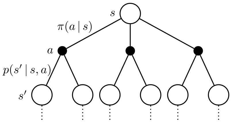
\[V^\pi(s) = \sum_a \pi(a \mid s) \sum_{s'} p(s' \mid s, a) [r(s, a) + \gamma V^\pi(s')]\]
The outer sum averages over the actions \(\pi\) may pick in \(s\). The inner sum averages over the possible responses of the environment. We know \(\pi(a \mid s)\) because \(\pi\) is given; neither \(p(s' \mid s,a)\) nor \(r(s,a)\) is known in general, unless we have a model.
The future unfolds as a tree, one level per time step. That tree is the backup diagram. The root is the current state; black disks are actions, weighted by \(\pi(a \mid s)\); from each action the environment branches to next states, weighted by \(p(s' \mid s,a)\). The same equation for \(Q^\pi\),
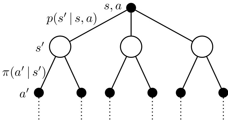
\[Q^{\pi}(s, a) = \sum_{s'} p(s' \mid s, a) \left[ r(s, a) + \gamma \sum_{a'} \pi(a' \mid s') Q^{\pi}(s', a') \right],\]
has the same diagram shifted by half a level: it alternates “environment, then policy” instead of “policy, then environment”.
When the dynamics are unknown we cannot expand the expectations, and are left with the compact forms
\[V^\pi(s) = \mathbb{E}_\pi \left[ R_{t+1} + \gamma V^\pi(S_{t+1}) \mid S_t = s \right],\] \[Q^\pi(s, a) = \mathbb{E}_\pi \left[ R_{t+1} + \gamma Q^\pi(S_{t+1}, A_{t+1}) \mid S_t = s, A_t = a \right].\]
This reframing is what unifies all value-based methods. They all estimate \(V^\pi\) or \(Q^\pi\) by traversing the backup diagram in some way, and the traversal is characterised by exactly two questions.
How deep? Do we expand the tree all the way to the end of the episode, or stop early and replace the rest with a current estimate of \(V^\pi\)?
Stopping early is bootstrapping. It is cheap and quiet, but part of the answer is a guess.
How wide? At each branching point, do we follow a single path by sampling, or expand all branches and average them with their probabilities?
Expanding all branches computes the expectation exactly, which requires knowing the model.
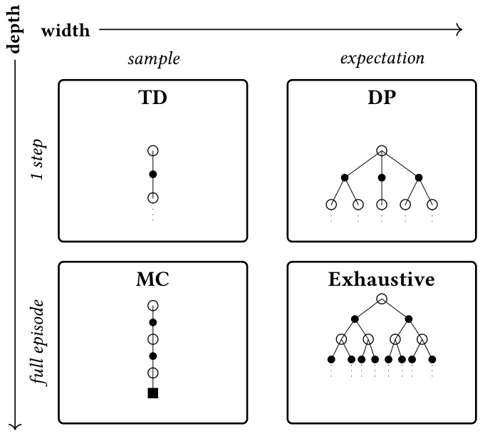
Different combinations of answers give different families of algorithms. The rest of this unit is a tour of that square.
Learning outcomes
- value-functions-and-backups Define \(V^\pi\) and \(Q^\pi\), write their Bellman equations, and place any value method on the depth/width backup spectrum.
Concepts
- value-function defines state-value \(V(s)\) and action-value \(Q(s,a)\) functions
- bellman-equation derives the Bellman equations and backup diagrams
Dynamic programming
Here we assume the dynamics of the environment, \(p(s' \mid s,a)\) and \(r(s,a)\), are known. The Bellman equation can then be applied directly, without sampling: at each state we expand all branches of the backup diagram and weight them by their true probabilities, exactly as we did for the \(4 \times 4\) grid. This is the full-width, one-step corner of the map.
That gives a system of \(|\mathcal{S}|\) equations in \(|\mathcal{S}|\) unknowns. It can be solved analytically, but rarely is in practice, because \(|\mathcal{S}|\) can be large. We instead iterate the Bellman operator:
\[L_\pi : \begin{cases} \mathbb{R}^{|\mathcal{S}|} & \to & \mathbb{R}^{|\mathcal{S}|} \\ V & \mapsto & R_\pi + \gamma P_\pi V \end{cases}\]
where \(R_\pi + \gamma P_\pi V\) is the right-hand side of the Bellman equation written in vector form.
Because \(L_\pi\) is a contraction mapping, the Banach fixed-point theorem guarantees that repeated application converges to \(V^\pi\). Convergence is not a matter of luck or of tuning; it is a property of the operator itself, and \(V^\pi\) is its unique fixed point.
Repeatedly applying \(L_\pi\) until it settles is the policy evaluation step. We now want to use \(V^\pi\) to find a better policy. The idea is simple: from state \(s\), set the new policy to take the action that looks best according to \(V^{\pi_k}\).
\[\pi_{k+1}(s) = \arg \max_a \sum_{s'} p(s' \mid s, a) [r(s, a) + \gamma V^{\pi_k}(s')]\]
That is the policy improvement step. Alternating evaluation and improvement gives the Policy Iteration algorithm.
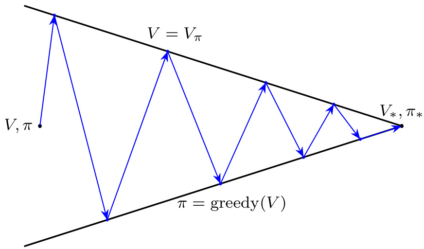
Read the two steps against the two axes of the previous section. Depth is one: we expand a single level and then substitute the current estimate \(V^{\pi_k}(s')\) for everything below it. Width is full: the sum over \(s'\) is the exact expectation, not a sample of it. Dynamic Programming is therefore the shallow, wide corner.
The method requires a perfect model of the environment, which is not available in most real-world problems. It also sweeps the entire state space on each pass. Its value to us is as the exact answer against which the sampling methods are measured — Monte Carlo and Temporal-Difference learning are what you do when you cannot expand the expectation.
For formal proofs, pseudocode and the Value Iteration algorithm, the book directs the reader to its supplementary material. We will not need them here.
Key ideas
- Dynamic Programming answers “how wide?” with all branches, using the known \(p(s' \mid s,a)\).
- Policy evaluation is iteration of \(L_\pi(V) = R_\pi + \gamma P_\pi V\); it converges because \(L_\pi\) contracts.
- Policy improvement is a greedy \(\arg\max\) over the one-step expansion.
- Policy Iteration alternates the two and converges to \((V^*, \pi^*)\).
- The model requirement is fatal in practice. Everything that follows relaxes it.
Learning outcomes
- dynamic-programming Run policy evaluation and policy improvement with a known model, and explain why the Bellman operator converges.
- value-functions-and-backups Define \(V^\pi\) and \(Q^\pi\), write their Bellman equations, and place any value method on the depth/width backup spectrum.
Concepts
- dynamic-programming details policy evaluation and policy improvement under known dynamics
- bellman-equation uses the exact Bellman operator to compute values without sampling
Monte Carlo methods
We now drop the assumption of known dynamics. Without \(p(s' \mid s,a)\) we can no longer compute the expectations in the Bellman equation. But an expectation can be estimated by sampling. So instead of computing \(V^\pi(s) = \mathbb{E}_\pi[G_t \mid S_t = s]\) directly, we gather experience in the environment and average the returns obtained after each visit to \(s\):
\[V^\pi(s) \approx \frac{1}{N(s)} \sum_{t: S_t = s} G_t,\]
where \(N(s)\) counts the visits to \(s\) across timesteps and episodes. On the backup diagram this is the opposite corner from Dynamic Programming: instead of expanding all branches one step deep, we sample a single path and follow it all the way to the end of the episode. This is Monte Carlo evaluation.
The update is usually written incrementally. On visiting \(S_t\) and observing the return \(G_t\):
\[V(S_t) \leftarrow V(S_t) + \alpha[G_t - V(S_t)],\]
with \(\alpha > 0\) a learning rate. Setting \(\alpha = 1/N(S_t)\) makes this exactly the running average above.
Control needs \(Q\), and \(Q\) needs exploration
Monte Carlo Control updates \(Q^\pi\) rather than \(V^\pi\) and improves the policy greedily, \(\pi_{k+1}(s) = \arg\max_a Q^{\pi_k}(s,a)\). The reason we estimate \(Q\) and not \(V\) is worth stating plainly: comparing actions through \(V^\pi\) would require summing over next states with \(p(s' \mid s,a)\), which we no longer have. \(Q^\pi\) absorbs that dependency. This is why \(Q^\pi\) was introduced in the first place.
A problem now appears that did not exist under Dynamic Programming. There, every action was implicitly tried through the expectation. Here, the only way to learn the value of an action is to actually take it. A purely greedy \(\pi_{k+1}\) will only ever pick the action that currently looks best; the others are never tried, their \(Q\)-values never update, and the policy gets stuck on whatever the initial estimates happened to be.
This is the exploration-exploitation dilemma, and it appears the moment the agent collects its own data. The fix is to never let the policy become fully greedy. With an \(\varepsilon\)-greedy policy the improvement step becomes:
\[ \pi_{k+1}(a \mid s) = \begin{cases} 1 - \epsilon + \frac{\epsilon}{|\mathcal{A}|} & \text{if } a = \arg\max_{a'} Q^{\pi_k}(s, a') \\ \frac{\epsilon}{|\mathcal{A}|} & \text{otherwise.} \end{cases} \]
A small \(\epsilon\) exploits aggressively but risks missing better actions; a large \(\epsilon\) explores broadly but wastes time on actions currently considered suboptimal. In practice \(\epsilon\) is often set to a small value such as \(0.1\), or decayed during training.
Algorithm - MC Control
1: init Q(s, a), pi eps-greedy with respect to Q
2: for each episode do
3:     collect s_0, a_0, r_1, ..., s_{T-1}, a_{T-1}, r_T ~ pi
4:     G <- 0
5:     for t = T-1, ..., 0 do
6:         G <- gamma*G + r_{t+1}
7:         Q(s_t, a_t) <- Q(s_t, a_t) + alpha*[G - Q(s_t, a_t)]
8:         pi(.|s_t) <- eps-greedy(Q(s_t, .))
9:     end for
10: end for
Notice the interleaving. The policy is updated right after each \(Q\) update, which does not respect the strict separation of evaluation and improvement that Dynamic Programming observed. We never wait for \(Q^{\pi_k}\) to be properly estimated before moving to \(\pi_{k+1}\). Taking new experience into account right away lets the policy improve faster.
Because \(\pi\) keeps evolving, returns collected long ago were generated by a policy that no longer matches the current one. Averaging them with equal weight, as \(1/N(s)\) would, biases the estimate toward the past. A constant \(\alpha\) gives more weight to recent returns, which is what we want when the policy itself is a moving target.
Monte Carlo Control has two drawbacks. It works only for episodic tasks, since we need episodes to terminate before returns can be computed. And the variance of the returns can be very high, especially for long episodes, which makes the estimates noisy and slow to converge. The next family of methods addresses both.
Learning outcomes
- monte-carlo-control Estimate values from complete sampled episodes and turn the estimates into control with \(\varepsilon\)-greedy action selection.
- bias-variance-spectrum Trade bias against variance with \(n\)-step returns, TD(\(\lambda\)) and GAE.
Concepts
- monte-carlo-methods presents model-free evaluation and control using complete episode returns
- value-function estimates state and action values by sample averaging
SARSA: on-policy TD control
What if, instead of waiting until the end of the episode, we used our current estimate of \(V^\pi\) to approximate the rest of the trajectory? That is Temporal-Difference (TD) learning, and SARSA is an instance of it.
TD resembles Monte Carlo in that it samples a single path through the backup diagram. It differs in going only one step deep and using the current estimate of \(V^\pi\) to fill in the rest. Filling in the rest with your own estimate is called bootstrapping.
After observing a single transition \((S_t, A_t, R_{t+1}, S_{t+1})\) we update:
\[V(S_t) \leftarrow V(S_t) + \alpha \left[ R_{t+1} + \gamma V(S_{t+1}) - V(S_t) \right]\]
The bracketed quantity is the TD error. It measures the discrepancy between the current estimate \(V(S_t)\) and a slightly better one built from a real reward \(R_{t+1}\) followed by our estimate of what comes next. We nudge \(V(S_t)\) to reduce it.
The target is now \(R_{t+1} + \gamma V(S_{t+1})\) rather than the full return \(G_t\), which addresses both of Monte Carlo’s drawbacks. Episodes no longer need to terminate. And the variance is lower, since the target depends on a single random reward and a single random transition rather than on the entire future. The cost is bias: the target contains \(V(S_{t+1})\), which is only an estimate. TD is therefore particularly sensitive to the initialisation of \(V\), and a badly initialised value function can take time to shed its bias.
The control counterpart works on \(Q\) rather than \(V\), giving SARSA:
\[Q(S_t, A_t) \leftarrow Q(S_t, A_t) + \alpha[R_{t+1} + \gamma Q(S_{t+1}, A_{t+1}) - Q(S_t, A_t)]\]
The name comes from the quintuple the update consumes: state, action, reward, next state, next action.
Algorithm - SARSA
1: Init Q(s, a), set pi eps-greedy with respect to Q
2: for each episode do
3:     observe s_0, sample a_0 ~ pi(.|s_0)
4:     for t = 0, 1, 2, ... until s_t terminal do
5:         take action a_t, observe r_{t+1}, s_{t+1}
6:         sample a_{t+1} ~ pi(.|s_{t+1})
7:         Q(s_t, a_t) <- Q(s_t, a_t)
8:                        + alpha*[r_{t+1} + gamma*Q(s_{t+1}, a_{t+1}) - Q(s_t, a_t)]
9:         pi(.|s_t) <- eps-greedy(Q(s_t, .))
10:    end for
11: end for
The action \(A_{t+1}\) in the target is the action the agent actually takes, sampled from the \(\varepsilon\)-greedy \(\pi\). Hold on to that. The next two sections turn on it entirely.
MC against TD on a random walk
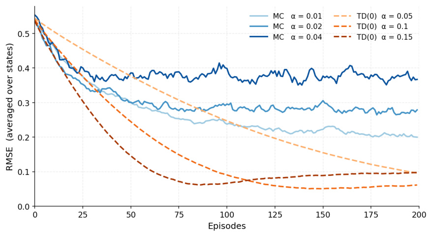
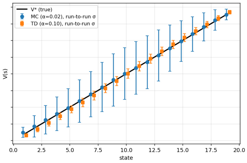
To see the difference, the book uses the 19-state random walk. The agent starts in the middle of a chain of 19 states and moves left or right uniformly at random. The leftmost end gives \(-1\), the rightmost gives \(+1\), every other transition gives \(0\). Both methods evaluate and follow the same random policy.

Convergence speed. Measured by RMS error against the true value function, TD converges much faster than MC.
Variance of updates. MC sees returns with far more variance than the TD targets, making its estimate noisier.
Variance across runs. TD estimates have much lower inter-run variance, because MC targets are full returns whose variance grows with episode length while TD targets depend on a single transition.
Propagation of rewards. TD propagates reward from the terminal states inward much more predictably.
This follows from bootstrapping, which exploits the Markov property. MC treats each state’s estimate independently and does not use the structure of the value function across states. The book draws the practical conclusion: use TD where the Markov property holds well, MC otherwise.
Learning outcomes
- td-control-updates Write and apply the SARSA and Q-learning update rules from a single transition.
- on-policy-vs-off-policy Distinguish on-policy from off-policy learning and predict the consequences for exploration safety and data reuse.
Concepts
- temporal-difference-learning introduces 1-step bootstrapping using the TD error
- sarsa formulates the on-policy SARSA control algorithm
Q-learning: off-policy TD control
Q-learning is another instance of TD, with one small but consequential change.
Recall SARSA’s target, \(R_{t+1} + \gamma Q(S_{t+1}, A_{t+1})\). Since \(\pi\) is \(\varepsilon\)-greedy, \(A_{t+1}\) is the greedy action most of the time and sometimes a random one. The target therefore reflects the value of \(\pi\) itself, exploration behaviour included. SARSA evaluates its own behaviour, and then tries to improve it.
That seems natural, since \(\pi\) is what we are running. But one can argue the other way. Exploration is added artificially for mechanical reasons. It is not intrinsic to the problem, and not ultimately something we want to optimise. We could ignore it when evaluating, while still using it to try actions and collect experience.
The general question is: from which policy should we sample the action \(a'\) used to build the target?
- SARSA, or on-policy TD control, uses the same policy \(\pi\) for acting and for evaluating.
- Off-policy TD control decouples the two. The action actually taken in the environment is sampled from a behaviour policy \(b\), with \(A_t \sim b(\cdot \mid S_t)\), while the action \(a'\) used to compute the target is sampled from the target policy \(\pi\), with \(a' \sim \pi(\cdot \mid S_{t+1})\).
The behaviour policy generates experience, so it must explore. The target policy is the one we evaluate and improve, and the one we ultimately care about.
The natural choice is \(\pi = \text{greedy}(Q)\) and \(b = \varepsilon\text{-greedy}(Q)\). That is Q-learning:
\[Q(S_t, A_t) \leftarrow Q(S_t, A_t) + \alpha \left[ R_{t+1} + \gamma \max_{a'} Q(S_{t+1}, a') - Q(S_t, A_t) \right]\]
The rest of the algorithm is identical to SARSA. Because the target is a sample of the Bellman optimality operator, we can also read Q-learning as directly estimating the optimal action-value function \(Q^*\).
Off-policy methods can learn from experience generated by any policy, not just the current one. Old experience collected under outdated policies remains valid training data. This matters enormously in deep RL, where data efficiency dominates — and it is why you have probably heard of Deep Q-learning but not of Deep SARSA.
Off-policy and offline are not the same thing. Off-policy RL learns from transitions generated by a different policy than the one being trained. Offline RL learns from a fixed dataset with no further environment interaction. Any offline method is therefore off-policy; the converse does not hold.
Learning outcomes
- td-control-updates Write and apply the SARSA and Q-learning update rules from a single transition.
- on-policy-vs-off-policy Distinguish on-policy from off-policy learning and predict the consequences for exploration safety and data reuse.
Concepts
- q-learning introduces off-policy TD control via max over next actions
- temporal-difference-learning applies 1-step bootstrapping toward the optimal Bellman target
Cliff Walking: the two behaviours side by side
The classic cliff walking environment illustrates the difference between on-policy and off-policy control during training, and it does so visibly.
The agent navigates a small grid from a start cell to a goal cell. The bottom row, except for the two endpoints, is a cliff. Stepping into it gives a reward of \(-100\) and sends the agent back to the start. Every other step gives \(-1\). The agent therefore wants to reach the goal as quickly as possible while avoiding the cliff. The optimal path goes just above the edge of the cliff and takes 13 steps.
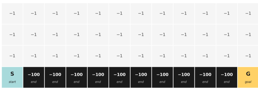
Both algorithms are trained with the same \(\varepsilon\)-greedy exploration, \(\epsilon = 0.1\), and the same learning rate. Tracking the sum of rewards collected per episode during training gives a result that surprises most readers the first time.
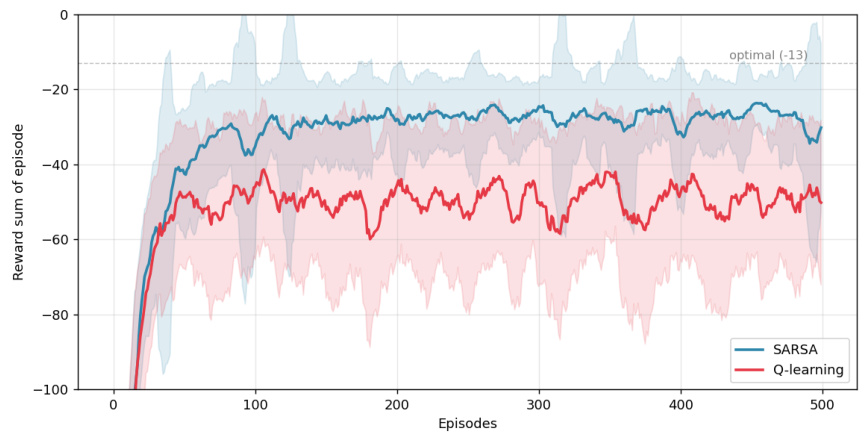
SARSA performs much better during training, although the policy it learns is worse than Q-learning’s.
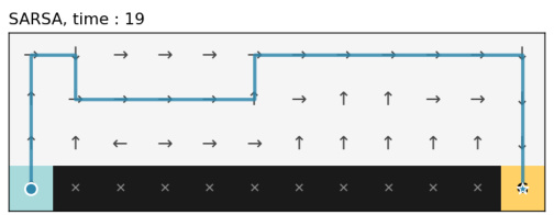
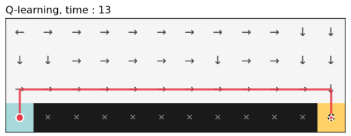
The explanation follows directly from the two targets.
Q-learning learned the optimal policy because it did not account for exploration during evaluation.
Every time an action was chosen randomly and led over the cliff, that outcome was absent from Q-learning’s target, which uses \(\max_{a'} Q(S_{t+1}, a')\) regardless of what was actually done.
SARSA learned a safer policy because those falls were in its target.
Its target uses the action actually taken, so the cost of the occasional exploratory step off the edge is baked into the values of the cells beside the cliff.
The lesson generalises beyond the gridworld. On-policy methods evaluate the policy you are actually running, noise and all. If exploration is intrinsic to deployment — a real robot that may behave imperfectly — the safer behaviour of SARSA may be preferable to the optimal-but-brittle path.
Learning outcomes
- on-policy-vs-off-policy Distinguish on-policy from off-policy learning and predict the consequences for exploration safety and data reuse.
- td-control-updates Write and apply the SARSA and Q-learning update rules from a single transition.
Concepts
- sarsa demonstrates SARSA learning a safer path due to on-policy exploration accounting
- q-learning demonstrates Q-learning converging to the optimal path along the cliff edge
Between MC and TD: \(n\)-step returns and TD(\(\lambda\))
We have seen two extremes. MC uses the full return \(G_t\); TD uses a one-step bootstrap \(R_{t+1} + \gamma V(S_{t+1})\). They sit at opposite ends of one spectrum with opposite trade-offs: MC has high variance but no bias, TD has low variance but introduces bias through bootstrapping. Can we interpolate?
\(n\)-step TD
Instead of bootstrapping after one step, sum \(n\) real rewards and bootstrap on the \(n\)-th next state. The \(n\)-step return is:
\[G_t^{(n)} = R_{t+1} + \gamma R_{t+2} + \dots + \gamma^{n-1} R_{t+n} + \gamma^n V(S_{t+n}).\]
The update rule is the TD one with \(G_t^{(n)}\) in place of the one-step target, \(V(S_t) \leftarrow V(S_t) + \alpha[G_t^{(n)} - V(S_t)]\). Setting \(n = 1\) recovers TD. Taking \(n\) large enough to reach the terminal state recovers MC. Intermediate values trade variance against bias: larger \(n\) uses more real rewards, so less bootstrapping bias, but accumulates more randomness.
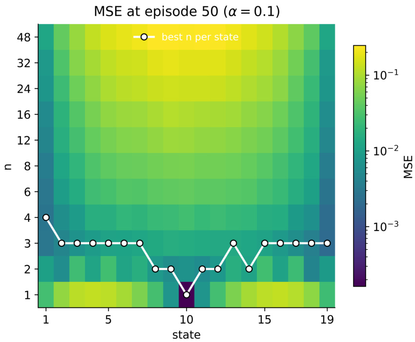
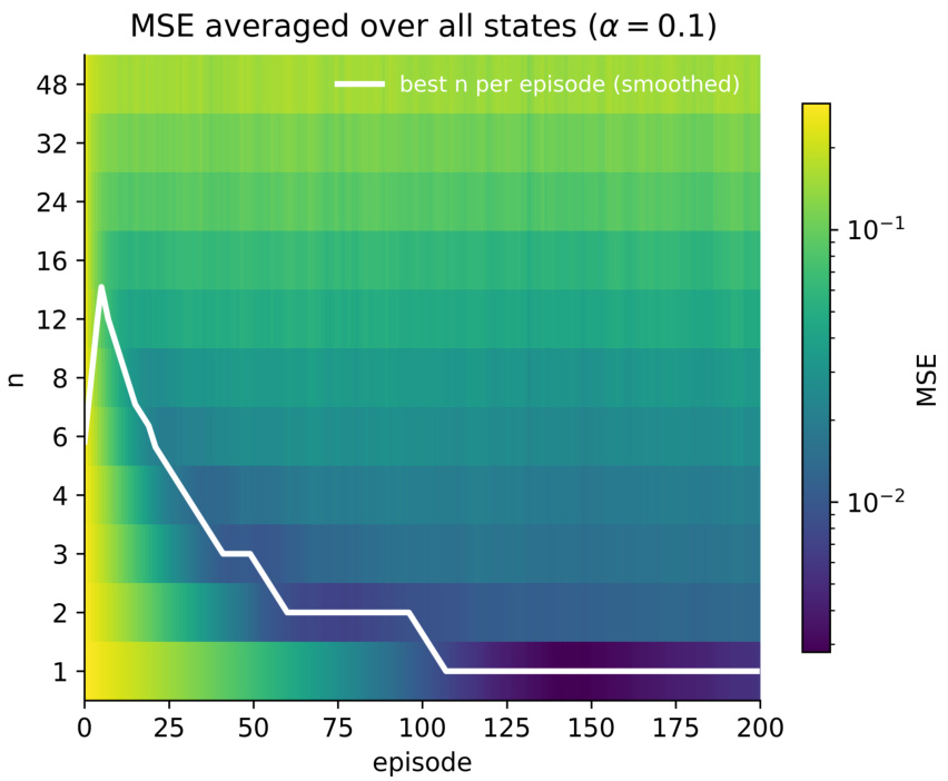
The important observation is that a single \(n\) is rarely optimal throughout. The best choice depends on both the state and the stage of training.
- Spatially. States whose neighbours have accurate value estimates can use a small \(n\), since the bootstrap \(V(S_{t+n})\) is trustworthy. States surrounded by poorly estimated values need a larger \(n\) to look past the biased bootstrap and reach real reward.
- Temporally. At the start, \(V\) is wrong everywhere, every bootstrap is biased, and a large \(n\) is preferable. As \(V\) converges the optimal \(n\) drifts down, because bias has been absorbed and variance becomes the dominant concern.
TD(\(\lambda\))
Rather than choosing, TD(\(\lambda\)) averages all \(n\)-step returns at once, weighted geometrically by \(\lambda \in [0,1]\):
\[G_t^\lambda = (1 - \lambda) \sum_{n=1}^{\infty} \lambda^{n-1} G_t^{(n)}.\]
- \(\lambda = 0\) gives TD(0), which is what we have been calling TD.
- Low values of \(\lambda\) give more weight to short-term returns, but are smoother than a fixed \(n\) because they still average over all \(n\).
- High values of \(\lambda\) give more weight to long-term returns.
- \(\lambda = 1\) gives MC.
Intuitively, TD(\(\lambda\)) hedges its bets in the bias-variance trade-off, which choosing a single \(n\) does not do. Averaging over all \(n\) removes the need to rely on one value. On the 19-state random walk this is not merely intuitive: TD(\(\lambda\)) is Pareto-superior to \(n\)-step TD, meaning no choice of \(n\) beats it on both bias and variance at once.
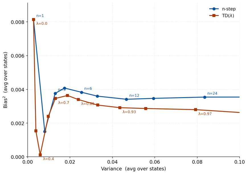
This idea is used extensively in modern RL, notably in Generalized Advantage Estimation (GAE), which uses the same target as TD(\(\lambda\)):
\[A_t^{\text{GAE}(\lambda)} = G_t^\lambda - V(S_t) = \sum_{k=0}^\infty (\gamma\lambda)^k \delta_{t+k},\]
where \(\delta_t = R_{t+1} + \gamma V(S_{t+1}) - V(S_t)\) is the TD error. We will carry this straight into policy optimisation later in the unit.
Key ideas
- Depth was never binary. \(n\)-step returns sweep it continuously from TD (\(n=1\)) to MC (\(n \to \infty\)).
- The best \(n\) varies across states and across training, so no fixed choice is right for long.
- TD(\(\lambda\)) averages every \(n\)-step return with weight \((1-\lambda)\lambda^{n-1}\), giving one knob for the whole spectrum.
- Empirically it dominates any single \(n\)-step estimator on the random walk.
- The same construction applied to advantages is GAE, which we meet again in policy optimisation.
Learning outcomes
- bias-variance-spectrum Trade bias against variance with \(n\)-step returns, TD(\(\lambda\)) and GAE.
- value-functions-and-backups Define \(V^\pi\) and \(Q^\pi\), write their Bellman equations, and place any value method on the depth/width backup spectrum.
Concepts
- td-lambda introduces \(n\)-step TD returns and TD(\(\lambda\)) geometric averaging
- temporal-difference-learning extends single-step TD bootstrapping to multi-step horizons
- monte-carlo-methods recovers Monte Carlo returns as the infinite-step, \(\lambda = 1\) limit
Deep Q-Networks
So far we have assumed that states and actions are discrete and few enough to enumerate, so that \(Q\) can be stored in a table and each \((s,a)\) updated independently. That assumption fails for two reasons.
- Many real problems have continuous state spaces, such as physics-based control tasks involving positions and velocities, or huge discrete ones, such as language models where the states are all possible token sequences. We could never visit every cell during training.
- In the tabular case each cell is learned in isolation, and the closeness between states is not exploited. We can usually expect the value function to be smooth across states, and would like to generalise from one state to its neighbours.
The fix is function approximation: replace the table with a parametric function \(Q_\theta(s,a)\) and learn \(\theta\). We typically use a neural network, which is where Deep Reinforcement Learning begins.
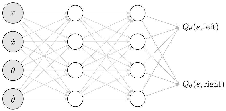
In principle any of the tabular algorithms could be extended this way. In practice value-based deep RL is dominated by Q-learning-style methods, for the data-efficiency reason of the previous sections. That is why every Deep Q-learning implementation you will encounter has a replay buffer \(\mathcal{D}\) storing past transitions that remain valid for training the current policy.
From an update rule to a regression
The tabular Q-learning update was a step toward the TD target \(y = R_{t+1} + \gamma \max_{a'} Q(S_{t+1}, a')\). With a parametric \(Q_\theta\) the natural analogue is to minimise the squared distance to that target by stochastic gradient descent:
\[\mathcal{L}(\theta) = \mathbb{E}_{(s,a,r,s') \sim \mathcal{D}} \left[ (y - Q_\theta(s,a))^2 \right], \qquad y = r + \gamma \max_{a'} Q_\theta(s', a').\]
Two complications separate this from standard supervised regression.
Consecutive transitions in a trajectory are highly correlated, which violates the i.i.d. assumption of SGD.
This is less problematic for off-policy methods, because we may sample from any past transition rather than the one just observed. Replay is legitimate precisely because Q-learning is off-policy.
The target \(y\) depends on \(\theta\), which we are updating.
The regression is chasing a target that moves every time we step.
Deep Q-learning (DQN) was historically the first algorithm to address these at scale and train a deep network to play Atari games at human level. Its main innovation is the target network, a separate copy \(Q_{\theta^-}\) used to compute targets:
\[y = r + \gamma \max_{a'} Q_{\theta^-}(s', a').\]
The target parameters \(\theta^-\) are held fixed and only synced to \(\theta\) every few thousand steps.
Algorithm - Deep Q-learning (DQN)
1: Initialize replay buffer D
2: Initialize theta at random; set theta- <- theta
3: for episode = 1, ..., M do
4:     Observe initial state s
5:     repeat
6:         a <- eps-greedy(Q_theta(s, .))
7:         Execute a, observe r, s'
8:         Store (s, a, r, s') in D
9:         Sample minibatch B from D
10:        for (s_j, a_j, r_j, s_j') in B do
11:            y_j <- r_j + gamma * max_{a'} Q_{theta-}(s_j', a')
12:        end for
13:        gradient step on loss (1/|B|) sum_j (y_j - Q_theta(s_j, a_j))^2
14:        s <- s'
15:        theta- <- theta every C steps
16:    until s is terminal
17: end forThe network produces one output per action and a \(\max\) is applied on top. A continuous action space has no such enumeration, so DQN as stated does not apply to it.
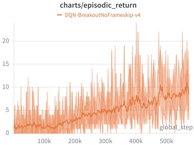
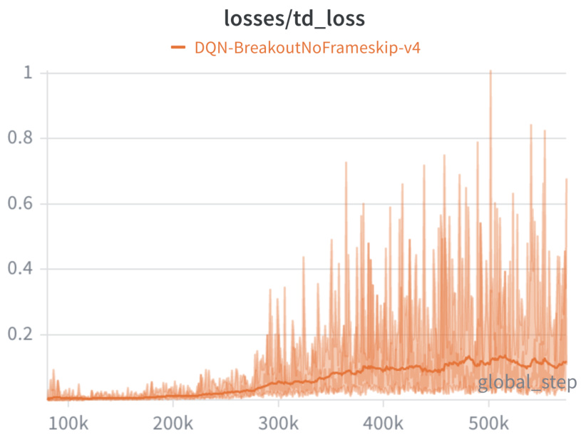
A core difficulty of RL training is the lack of reliable signal. The reward curve is noisy, from both environment stochasticity and \(\varepsilon\)-greedy exploration, and it is only indirectly related to the TD error we actually optimise. The TD loss is no better: the regression target is a moving quantity that changes as the policy improves and visits new states, so the TD loss is not the value of any fixed objective. It may rise while training is healthy, because a better policy is exploring new regions of the state space, and it may fall while training is stuck on a degenerate policy. Contrast a supervised language-model loss, which can be near-perfectly smooth for a trillion-parameter model.
Learning outcomes
- deep-q-networks Replace the Q-table with a neural network and stabilise the result with a replay buffer and a target network.
- on-policy-vs-off-policy Distinguish on-policy from off-policy learning and predict the consequences for exploration safety and data reuse.
Concepts
- deep-q-network explains Deep Q-learning, replay buffers, and target networks
- q-learning adapts tabular Q-learning to parametric function approximation
Policy optimisation: the setup
In the value-based half of this unit the policy was never the object of optimisation. We tried to make \(Q_\theta\) satisfy a Bellman equation, and recovered a policy implicitly as \(\arg\max_a Q_\theta(s,a)\). We now take a different route: parameterise the policy and learn its parameters directly. This is the domain of policy optimisation methods.
We write the policy as \(\pi_\theta(a \mid s)\), typically a neural network mapping a state to a distribution over actions.
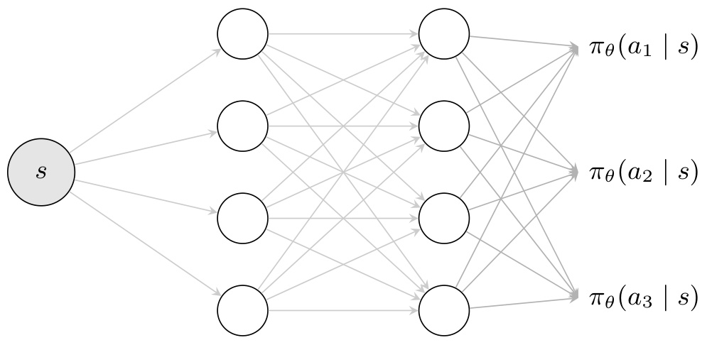
This handles continuous action spaces immediately, by outputting the parameters of a continuous distribution — the mean and variance of a Gaussian, for instance. That is a genuine advantage over the value-based route, where the \(\max\) over actions demanded an enumerable action set.
We frame learning as the optimisation of
\[J(\theta) = \mathbb{E}_{\tau \sim \pi_\theta} [G(\tau)]\]
where \(\tau = (S_0, A_0, R_1, S_1, A_1, R_2, \ldots, S_T)\) is a trajectory sampled by following \(\pi_\theta\) in the environment and \(G(\tau) = \sum_{t=0}^{T-1} \gamma^t R_{t+1}\) is its discounted return. The problem is then \(\theta^* = \arg\max_\theta J(\theta)\).
In the value-based chapter the loss we minimised was only a proxy: a squared TD error, whose value tells us little about how well the agent performs. Here \(J(\theta)\) is the quantity we care about, the expected return, and we differentiate it directly.
The difficulty is immediate, and it is worth naming before we attack it. \(\theta\) appears in the distribution we are averaging over, not merely in the thing being averaged. Differentiating under the integral therefore does not directly yield an expectation, and without an expectation there is nothing to estimate from samples.
Two families answer this differently, and we will take them in order.
- Policy gradient methods compute \(\nabla_\theta J(\theta)\) via the policy gradient theorem and apply gradient ascent. REINFORCE is the representative.
- Trust region methods build a surrogate objective that locally approximates \(J\) and optimise it within a region where the approximation holds. PPO is the representative.
Learning outcomes
- policy-gradient-theorem Derive the policy gradient and cut its variance with reward-to-go and a learned baseline.
Concepts
- policy-gradient-theorem sets up the expected return objective \(J(\theta)\) for policy parameter optimisation
Policy gradients and variance reduction
The policy gradient theorem expresses \(\nabla_\theta J(\theta)\) in a form estimable from samples. Its weaker form states:
\[\nabla_\theta J(\theta) = \mathbb{E}_{\tau \sim \pi_\theta} \left[ G(\tau) \sum_{t=0}^{T-1} \nabla_\theta \log \pi_\theta (A_t \mid S_t) \right].\]
The formula reads naturally once decomposed.
- \(\nabla_\theta \log \pi_\theta(A_t \mid S_t)\) is the direction in parameter space that makes action \(A_t\) more likely in state \(S_t\).
- Summing these directions over all timesteps gives the direction that makes the whole trajectory \(\tau\) more likely.
- Scaling by the scalar \(G(\tau)\) decides the sign. If the trajectory was good, we step in the direction that makes all of its actions more likely. If it was bad, we step the other way.
Approximating by sampling \(N\) trajectories gives Simple Policy Gradient (SPG), with the estimator \(\hat{g} \leftarrow \frac{1}{N} \sum_{i} G(\tau_i) \sum_{t} \nabla_\theta \log \pi_\theta(a_t^{(i)} \mid s_t^{(i)})\) and the ascent step \(\theta \leftarrow \theta + \alpha \hat{g}\). It is correct, and extremely noisy.
A typical PyTorch implementation writes
loss = -(policy(obs).log_prob(act)*weight).mean()with weight equal to \(G(\tau)\) for SPG. Two warnings come with it. Its numerical value carries no information about how well the policy performs: grad(loss) points opposite to \(\nabla_\theta J(\theta)\), but the value of loss is not \(J(\theta)\). And even as a gradient signal it is valid only at the parameters used to collect the data. The first gradient step on a batch is correct; after it, \(\theta\) has moved and grad(loss) no longer estimates \(\nabla_\theta J(\theta)\). This makes policy gradient methods inherently on-policy, and part of why they are less data-efficient than the off-policy Q-learning methods — no replay buffer is possible.
First reduction: reward-to-go
Under the weak form, the same \(G(\tau)\) weights every action in the trajectory. That does not really make sense. For action \(A_t\), the return \(G(\tau)\) contains rewards \(R_1, \ldots, R_t\) collected before \(A_t\) was taken. Those cannot have been caused by it. They have zero expectation and only add variance.
The reward-to-go form replaces \(G(\tau)\) with \(G_t\), the same cumulative discounted reward from time \(t\) that we used throughout the value-based half:
\[\nabla_{\theta} J(\theta) = \mathbb{E}_{\tau \sim \pi_{\theta}} \left[ \sum_{t=0}^{T-1} G_t \nabla_{\theta} \log \pi_{\theta}(A_t \mid S_t) \right].\]
Both forms are valid and yield the same expectation, since the past rewards contribute only variance. This refinement is REINFORCE, which is SPG with \(G(\tau)\) replaced by \(G_t\).
Second reduction: a baseline
REINFORCE is still noisy. Subtract a baseline \(b(S_t)\) from the return:
\[\nabla_\theta J(\theta) = \mathbb{E}_{\tau \sim \pi_\theta} \left[ \sum_{t=0}^{T-1} (G_t - b(S_t)) \nabla_\theta \log \pi_\theta(A_t \mid S_t) \right]\]
As long as \(b(S_t)\) does not depend on \(A_t\), the expectation is unchanged and the estimator stays unbiased for any \(b\). The variance, however, depends on it very much.
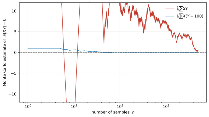
The book makes this concrete with a scalar example. Let \(X = \pm 1\) with probability \(1/2\) each and \(Y = 100 \pm 1\), and estimate \(\mu = \mathbb{E}[XY] = \mathbb{E}[X]\mathbb{E}[Y] = 0\).
- The naive estimator \(\hat{\mu} = XY\) takes values \(\pm 99\) or \(\pm 101\), so its variance is \(\frac{1}{4}(99^2 + 101^2 + 99^2 + 101^2) = 10{,}001\).
- The baseline-subtracted \(\hat{\mu}_b = X(Y - 100)\) still has expectation zero, but takes values \(\pm 1\), so its variance is \(\frac{1}{4}(1+1+1+1) = 1\).
\(Y\) has a large mean and a small fluctuation. Multiplying it by a centred \(X\) amplifies that mean into a \(\pm 100\) swing, even though the mean carries no information about the quantity of interest — it is killed in expectation by \(\mathbb{E}[X] = 0\). Subtracting the mean of \(Y\) removes the parasitic swing and keeps the useful signal. Transpose the argument with \(X\) playing \(\nabla_\theta \log \pi_\theta(A_t \mid S_t)\), which is centred, and \(Y\) playing \(G_t\), which has a large mean and a smaller action-dependent fluctuation.
The natural choice is \(b(S_t) = V^{\pi_\theta}(S_t)\), the mean return from \(S_t\) under \(\pi_\theta\). We increase the probability of an action in proportion to how much better than expected it turned out to be. That quantity is the advantage:
\[A_t = G_t - V^{\pi_\theta}(S_t).\]
Chapter 3 already told us how to estimate \(V^{\pi_\theta}\), so we introduce a second network \(V_\phi\) trained alongside \(\pi_\theta\). The policy network is the actor, the value network the critic, and the family is actor-critic. The resulting algorithm is Vanilla Policy Gradient (VPG): the actor steps along \(\frac{1}{N}\sum_i \sum_t A_t^{(i)} \nabla_\theta \log \pi_\theta(a_t^{(i)} \mid s_t^{(i)})\) while the critic descends the squared error \(\frac{1}{2}(G_t^{(i)} - V_\phi(s_t^{(i)}))^2\).
Third reduction: GAE
\(A_t = G_t - V(S_t)\) is unbiased when \(V\) is correct, but inherits the high variance of \(G_t\), itself a single Monte Carlo sample of a long stochastic sum. We trade some of that variance for bias exactly as we did going from MC to TD. The one-step estimate is the TD error, \(A_t^{(1)} = R_{t+1} + \gamma V(S_{t+1}) - V(S_t) =: \delta_t\); the \(k\)-step estimate is
\[A_t^{(k)} = \sum_{l=0}^{k-1} \gamma^l R_{t+l+1} + \gamma^k V(S_{t+k}) - V(S_t),\]
and as \(k\) grows to \(T - t\) we recover the Monte Carlo advantage. Rather than picking one \(k\), the Generalized Advantage Estimator takes the exponentially weighted average of all of them:
\[A_t^{\text{GAE}} = (1-\lambda)\left(A_t^{(1)} + \lambda A_t^{(2)} + \lambda^2 A_t^{(3)} + \cdots\right) = \sum_{l=0}^{\infty} (\gamma \lambda)^l \delta_{t+l}.\]
Both \(\gamma\) and \(\lambda\) control the trade-off, but not in the same way: \(\gamma\) reduces variance by down-weighting all future rewards and \(\gamma < 1\) introduces bias, whereas \(\lambda < 1\) introduces bias only when \(V\) is poorly estimated. In practice \(\lambda\) is usually set around \(0.95\), and GAE has become the default advantage estimator in modern policy gradient implementations. It costs one backward pass through the trajectory, using
\[A_{t}^{\mathrm{GAE}} = \delta_{t} + \gamma \lambda A_{t+1}^{\mathrm{GAE}}, \qquad A_T^{\mathrm{GAE}} = 0.\]
Because \(A_t^{\mathrm{GAE}} = G_t^\lambda - V_\phi(S_t)\), the \(\lambda\)-return target for the critic comes essentially for free, and it is common to switch the critic to it as well. The stop-gradient operator sg marks the target as a constant during differentiation.
On CartPole the four estimators rank as expected: SPG below REINFORCE below VPG in performance, and in the reverse order for relative inter-run variance.
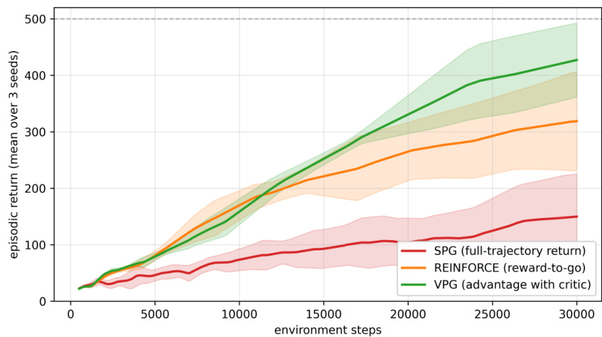
Sampling many trajectories at a fixed iteration and plotting one component of the gradient shows the variance falling monotonically from SPG through to VPG with GAE. The means of the first three coincide, because all three are unbiased; VPG with GAE sits elsewhere, because \(\lambda < 1\) introduces bias.
Learning outcomes
- policy-gradient-theorem Derive the policy gradient and cut its variance with reward-to-go and a learned baseline.
- bias-variance-spectrum Trade bias against variance with \(n\)-step returns, TD(\(\lambda\)) and GAE.
Concepts
- policy-gradient-theorem derives weak and reward-to-go forms of the policy gradient theorem
- value-function introduces critic baseline subtraction to form the advantage function
- generalized-advantage-estimation introduces GAE for exponentially weighted multi-step advantage estimation
- td-lambda uses TD(\(\lambda\)) mechanisms to derive GAE advantages and \(\lambda\)-return critic targets
Trust region methods and PPO
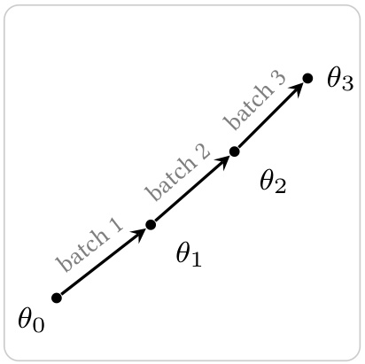
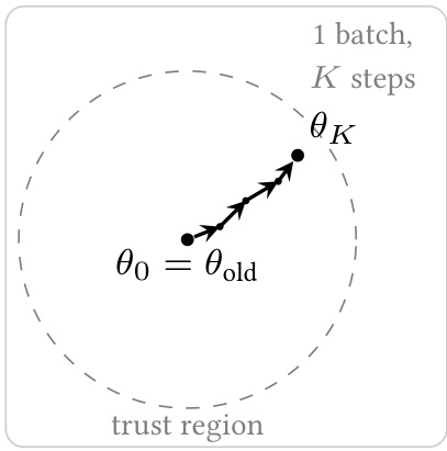
The algorithms so far estimated \(\nabla_\theta J(\theta)\) and applied gradient ascent. Trust region methods take a different starting point. Rather than differentiating \(J\), we look at the difference \(J(\theta) - J(\theta_{\text{old}})\) between a candidate new policy and the current one, and find that it admits a form approximable by a surrogate \(L_{\theta_{\text{old}}}(\theta)\) estimable from rollouts of \(\pi_{\theta_{\text{old}}}\) alone. The surrogate is accurate only in a neighbourhood of \(\theta_{\text{old}}\) — hence trust region, the region around \(\theta_{\text{old}}\) in which we trust our surrogate.
The payoff is extracting more from each batch. We now have an explicit objective we can optimise over several steps, so long as we stay inside the region. Policy gradients had to be conservative: nothing in theory justified a second gradient step on the same batch.
The performance difference lemma
The starting point is an exact identity relating the returns of two policies. For any \(\pi_\theta\) and \(\pi_{\theta_{\text{old}}}\):
\[J(\theta) - J(\theta_{\text{old}}) = \frac{1}{1 - \gamma} \mathbb{E}_{s \sim d^{\pi_\theta}, a \sim \pi_\theta} \left[ A^{\pi_{\theta_{\text{old}}}}(s, a) \right]\]
where \(d^\pi(s)\) is the normalised state visitation distribution induced by \(\pi\). The difference in performance between the two policies is obtained by evaluating the new policy under the old critic. To make \(\pi_\theta\) better than \(\pi_{\theta_{\text{old}}}\), we want \(\pi_\theta\) to put mass on actions with positive advantage under \(\pi_{\theta_{\text{old}}}\).
The identity is exact but not yet usable. The expectation is over the visitation distribution of the new policy, which we cannot sample from without rolling out \(\pi_\theta\) — and the whole point is to choose \(\theta\) before a new rollout. So we build a surrogate in two steps.
State distribution approximation. Swap \(d^{\pi_\theta}\) for \(d^{\pi_{\theta_{\text{old}}}}\), giving \(L_{\theta_{\text{old}}}(\theta) := \frac{1}{1-\gamma}\mathbb{E}_{s \sim d^{\pi_{\theta_{\text{old}}}}, a \sim \pi_\theta}[A^{\pi_{\theta_{\text{old}}}}(s,a)]\).
The approximation error grows with how much \(\pi_\theta\) visits different states than \(\pi_{\theta_{\text{old}}}\). This one swap is what dictates the existence of a trust region.
Importance sampling. The expectation still samples actions from \(\pi_\theta\), so rewrite it against \(\pi_{\theta_{\text{old}}}\):
\[L_{\theta_{\mathrm{old}}}(\theta) = \frac{1}{1 - \gamma} \mathbb{E}_{s \sim d^{\pi_{\theta_{\mathrm{old}}}},\, a \sim \pi_{\theta_{\mathrm{old}}}} \left[ \frac{\pi_{\theta}(a \mid s)}{\pi_{\theta_{\mathrm{old}}}(a \mid s)} A^{\pi_{\theta_{\mathrm{old}}}}(s, a) \right]\]
Importance sampling. To estimate an expectation under \(p\) when we can only sample from \(q\), use \(\mathbb{E}_{x \sim p}[f(x)] = \mathbb{E}_{x \sim q}\left[\frac{p(x)}{q(x)} f(x)\right]\), valid as long as \(q(x) > 0\) wherever \(p(x) > 0\). The ratio corrects the bias introduced by sampling from the wrong distribution.
Everything is now estimable from a batch collected by \(\pi_{\theta_{\text{old}}}\). But we may trust \(L_{\theta_{\text{old}}}(\theta)\) only while \(\pi_\theta\) stays close to \(\pi_{\theta_{\text{old}}}\). If we naively maximise the surrogate to convergence, we land on a \(\theta\) for which the swap \(d^{\pi_\theta} \to d^{\pi_{\theta_{\text{old}}}}\) is inaccurate, and for which the actual return \(J(\theta)\) may even drop. Hence the constrained problem \(\max_\theta L_{\theta_{\text{old}}}(\theta)\) subject to \(\pi_\theta \approx \pi_{\theta_{\text{old}}}\).
Different ways of enforcing closeness give different algorithms. TRPO uses an explicit KL constraint \(\mathbb{E}_{s}[D_{\text{KL}}(\pi_{\theta_{\text{old}}} \parallel \pi_\theta)] \leq \delta\), solved with a conjugate-gradient step on a quadratic approximation of the KL. It works, but is heavy to implement and to scale.
PPO’s clipped objective
Proximal Policy Optimization replaces that constraint with a much simpler proxy:
\[L^{\mathrm{CLIP}}(\theta) = \mathbb{E}_{\pi_{\theta_{\mathrm{old}}}} \left[ \min \left( \rho_t(\theta) \hat{A}_t, \operatorname{clip}(\rho_t(\theta), 1 - \epsilon, 1 + \epsilon) \hat{A}_t \right) \right]\]
where \(\rho_t(\theta) = \pi_\theta(A_t \mid S_t) / \pi_{\theta_{\mathrm{old}}}(A_t \mid S_t)\) is the importance ratio, \(\hat{A}_t\) is an advantage estimator (typically GAE), and \(\epsilon\) is a small constant, commonly \(0.1\) or \(0.2\), called the clip parameter.
The intuition is to limit how far each action can be pushed.
- If \(\hat{A}_t > 0\) we want to increase \(\pi_\theta(A_t \mid S_t)\), so \(\rho_t\) tends to grow. The clip caps the gain at \(\rho_t = 1 + \epsilon\); past that, the gradient is zero.
- If \(\hat{A}_t < 0\) we want to decrease it, so \(\rho_t\) tends to shrink. The clip caps the loss at \(\rho_t = 1 - \epsilon\).
- When \(\rho_t\) drifts outside the region against the sign of \(\hat{A}_t\) — say \(\rho_t < 1-\epsilon\) with \(\hat{A}_t > 0\) — the \(\min\) selects the unclipped term, so the gradient remains non-zero and pulls the policy back.
This is a soft trust region: the policy is softly prevented from moving too far on any single sample. PPO then performs several gradient steps on the same batch, typically around five epochs. As updates accumulate, ratios start hitting the clip and the gradient on those samples is zeroed, which slows the drift between \(\theta\) and \(\theta_{\text{old}}\). The rest of the algorithm is VPG with GAE, with \(\theta_{\text{old}}\) and the old log-probabilities cached before the epoch loop begins.
The very first gradient step of PPO, for which \(\rho_t = 1\) everywhere, recovers VPG’s policy gradient with advantages — even though the derivation went through the performance difference lemma rather than the policy gradient theorem.
And although PPO reuses a batch collected by a previous policy, we still mostly call it an on-policy method, since the surrogate is valid only for policies close enough to the one that produced the data. The number of gradient steps per iteration is also not \(K\) but \(K \times\) the number of minibatches, since each epoch shuffles and splits the batch.
What happens without the clip
On CartPole, VPG and PPO are compared for robustness to reusing one batch over \(K \in \{1, 4, 16\}\) epochs, with each batch split into 8 minibatches.
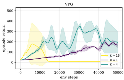
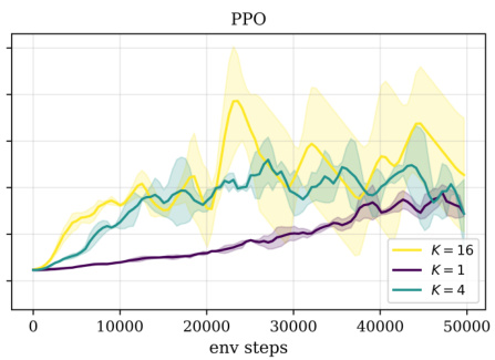
\(K = 1\) gives near-identical performance, for the reason just noted. The divergence at larger \(K\) is explained by the cumulative approximate KL divergence between the current policy and the data-generating policy, measured per minibatch step within a single iteration: PPO’s stays bounded, VPG’s explodes.
One might argue that a smaller step size would let VPG reuse batches too. It would not, or not reliably. A smaller step controls drift in parameter space, whereas the surrogate’s approximation \(d^{\pi_\theta} \approx d^{\pi_{\theta_{\text{old}}}}\) requires closeness in policy space, which closeness in parameter space does not guarantee. PPO limits drift in policy space directly, by stopping the gradient on actions that have already drifted too far while still making progress on the rest of the batch.
Key ideas
- The performance difference lemma is exact but samples the new policy’s state distribution.
- Swapping in the old state distribution creates a surrogate, and the swap’s error is what defines the trust region.
- Importance sampling makes the surrogate estimable from old rollouts.
- PPO clips the ratio to \([1-\epsilon, 1+\epsilon]\), zeroing the gradient once a sample has drifted too far.
- That is what makes several epochs per batch safe, and PPO the workhorse of modern RL.
Learning outcomes
- trust-region-and-ppo Justify a trust region from the performance difference lemma and implement PPO’s clipped surrogate objective.
- policy-gradient-theorem Derive the policy gradient and cut its variance with reward-to-go and a learned baseline.
- on-policy-vs-off-policy Distinguish on-policy from off-policy learning and predict the consequences for exploration safety and data reuse.
Concepts
- proximal-policy-optimization presents PPO’s clipped surrogate objective and compares it with VPG
- generalized-advantage-estimation uses GAE advantages as weights inside the PPO surrogate loss
What you can now do, and what comes next
Four ideas carry the whole unit, and each is worth stating with its consequence.
All value-based methods are one Bellman backup, traversed differently.
Depth decides whether you bootstrap after a step or roll to the end; width decides whether you take the exact expectation or a sample. DP, MC and TD are corners of that square, not rival philosophies.
The bias-variance trade-off is the axis every estimator sits on.
MC has no bias and high variance; one-step TD reverses that. TD(\(\lambda\)) and GAE refuse the choice by averaging all \(n\)-step returns geometrically, and dominate any single \(n\) on the random walk.
On-policy and off-policy is a distinction about whose data you may use.
SARSA and VPG evaluate the policy they are running, exploration noise included, which is why SARSA walks away from the cliff. Q-learning and DQN evaluate the greedy policy, which is why a replay buffer is available to them at all.
A surrogate objective is only as good as the region it is trusted in.
The policy gradient’s coded “loss” is valid at exactly one point in parameter space. PPO’s clipped ratio buys a region instead of a point, which is what makes multiple epochs per batch both safe and worthwhile.
Concretely, you can now write Bellman equations and place a method on the backup map; run policy evaluation and improvement with a model and estimate values without one; apply the SARSA and Q-learning updates and explain Cliff Walking from first principles; trade bias against variance with \(n\)-step returns, TD(\(\lambda\)) and GAE; build DQN with a replay buffer and a target network; derive the policy gradient and reduce its variance; and justify and implement PPO’s clipped trust region.
III RL at Scale applies all of this where the environment is a language model or a board game. Post-training moves from RLHF, which optimises human preferences and invites reward hacking, to RLVR, which uses deterministic verifiers on mathematics and STEM tasks — with GRPO dropping the critic you have just learned to build in favour of a group-sampled baseline. You will also meet the systems side: separate trainer and inference GPU fleets, asynchronous rollouts, and importance-sampling corrections for the off-policy drift that creates. That unit closes with AlphaGo Zero, where search is distilled back into a fast policy network.
References
- The Little Book of Reinforcement Learning, Alexandre Torres Leguet, 2026 — Link — Page 40-111