Lecture notes — III RL at scale
ver. 1.0.0, iii_rl_at_scale
ver. 1.0.0 · 2026-08-22 10:31:49
Where we are
In II Diving Deeper you built the algorithms. You wrote \(V^\pi\) and \(Q^\pi\) and their Bellman equations, placed every value method on the depth/width map, ran dynamic programming, Monte Carlo, SARSA and Q-learning, traded bias against variance with \(n\)-step returns, TD(\(\lambda\)) and GAE, replaced the Q-table with a network in DQN, derived the policy gradient, and closed with PPO’s clipped trust region.
This unit adds no new family. It watches those methods run at scale, in the two settings that made reinforcement learning famous: post-training a large language model, and AlphaGo Zero. Our source is Part III of The Little Book of Reinforcement Learning — Chapter 5, Chapter 6, and the book’s conclusion.
Nothing here is a new idea. It is the old ideas under pressure.
What you will be able to do
post-training-regimes— Distinguish SFT, RLHF and RLVR as post-training regimes, and say what each optimises and where each fails.llm-generation-as-mdp— Formalise token generation as an MDP and identify the state, action, transition and reward of an RLVR run.grpo— Explain how GRPO removes the critic by using a group of sampled completions as its baseline.rlvr-refinements— Evaluate the practical refinements to GRPO — entropy targeting, length penalties, dynamic sampling and sequence-level objectives.rl-infrastructure— Describe an RLVR training system: separate trainer and inference fleets, and the importance-sampling corrections their drift demands.sft-rl-continuum— Explain how SFT and RL relate as objectives, and describe the hybrid methods that sit between them.alphago-zero-loop— Explain AlphaGo Zero as policy iteration where MCTS is the improvement operator and self-play rollouts are the evaluation.self-play-and-test-time-compute— Explain why zero-sum self-play converges rather than collapses, and what a task needs before AlphaZero transfers to it.unifying-patterns— Identify the recurring patterns — credit assignment, bias-variance, moving distributions and data staleness — in any RL algorithm you meet.
What we will cover
- Reinforcement Learning with Verifiable Rewards (RLVR) — training against a mechanical, ground-truth verifier rather than a learned preference model.
- Group Relative Policy Optimization (GRPO) — a critic-free policy optimisation method that takes its baseline from a group of completions sampled for one prompt.
- High-entropy forking tokens — the positions where the model is uncertain, and where RLVR updates land hardest.
- Sequence-level policy optimization — treating a whole response as a single action, and the length-normalised importance ratio that keeps it stable.
- Asynchronous RLVR infrastructure and mismatch correction — decoupled trainer and inference fleets, and the importance ratios that pay for decoupling them.
- On-Policy Distillation — sampling from the student, supervising with a teacher.
- AlphaGo Zero self-play and MCTS policy iteration — search as the improvement step, network fitting as the evaluation step.
- Test-time compute — spending computation at inference to act better than a single forward pass allows.
Opening: where RL is actually used
Everything you have built so far was demonstrated on general problems — gridworlds, control tasks, small discrete environments. This unit applies the toolkit to two specific systems, and the interest lies in what breaks when the scale changes.
The first setting is RL \(\times\) LLMs. A pretrained language model is a very powerful conditional distribution over text. The book calls this the base model. It encodes a great deal of knowledge, but its behaviour is hard to predict and control, which makes that knowledge difficult to leverage. Fine-tuning is how the field extracts it, and since late 2022 that has been one of the central efforts in the field.
The second setting is AlphaGo Zero. The book’s stated aim in Chapter 6 is to give a high-level overview of the algorithm under the prism of the concepts built through the book. Its warning is worth repeating: you will find the ingredients familiar, but assembled in a quite different way from the value-based and policy-based families.
Three things are worth fixing before we begin.
The algorithms do not change; the constraints do. PPO becomes GRPO because a critic the size of the policy will not fit, not because the mathematics demanded it.
At scale, an algorithmic choice and an engineering choice stop being separable.
The environment can be a token stream. Generation is an MDP, and once you see it as one, every tool from II Diving Deeper applies unchanged.
Search can be an improvement operator. AlphaGo Zero puts a tree search where policy iteration puts a greedy
argmax, and trains the network to imitate the result.
We close the unit — and the module — by naming the patterns common to everything you have seen, and by marking the parts of the field this module did not enter.
Learning outcomes
- post-training-regimes Distinguish SFT, RLHF and RLVR as post-training regimes, and say what each optimises and where each fails.
- alphago-zero-loop Explain AlphaGo Zero as policy iteration where MCTS is the improvement operator and self-play rollouts are the evaluation.
- unifying-patterns Identify the recurring patterns — credit assignment, bias-variance, moving distributions and data staleness — in any RL algorithm you meet.
From SFT to RLHF to RLVR
A base model predicts the next token. Making it useful takes post-training, and the book distinguishes three regimes.
Supervised fine-tuning (SFT) is the most direct option. You collect demonstrations of the desired behaviour and train the model to imitate them. It is simple to implement and somewhat effective, but it requires demonstrations. RL needs none — only a reward function that scores model outputs and lets the model search for behaviour that scores well.
That difference matters for two reasons the book states plainly. RL can learn behaviour that was never demonstrated, such as decomposing a problem, considering alternatives, or checking its own work. And because the signal comes from a reward rather than a fixed human-written target, RL can in principle push models past the level of any specific human demonstrator.
Two generations of RL training for LLMs have emerged.
First generation: alignment (RLHF). Around 2022, RL was used to turn a base model into a chatbot or assistant. Reinforcement Learning with Human Feedback first trains a reward model to predict human preferences between two model outputs, then fine-tunes the base model with RL against that reward — reinforcing the tokens that led to highly-rewarded sequences. The recipe was very effective, and behind the success of products like ChatGPT.
It turned out RL was not strictly necessary to such alignment procedures.
Second generation: reasoning (RLVR). Starting in 2024, RL is used to train models in environments with verifiable rewards. The most common setup gives the model maths problems and rewards it for producing the correct numerical answer.
RLHF’s limitation is where it was constrained: by how reliable the reward model was, and by what it actually rewarded. Predicting human preferences is a quite shallow signal determined mostly by tone and style. It gives the model no incentive to reason, plan, or develop any new capability.
RLVR — Reinforcement Learning with Verifiable Rewards — replaces that learned proxy with a mechanical check. A byproduct of the setup is that it teaches the model thinking actions: planning, decomposing a problem, backtracking, self-checking. Verifiable rewards are natural on STEM tasks, where correctness can be checked mechanically, and much harder to construct for open-ended tasks like creative writing.
The consequence is one of scale. The RLVR reward is more interesting to optimise against and more robust to reward hacking, which makes it practical to run RLVR at much larger scale than RLHF — often approaching a non-trivial fraction of pretraining, more than \(10\%\).
It has not been eliminated. It has been moved. A deterministic verifier cannot be flattered, but as §Beyond GRPO will show, the model can still find pressure to exploit in whatever the objective incidentally rewards — response length, for instance.
The rest of Chapter 5, and the rest of our LLM sections, concerns RLVR.
Learning outcomes
- post-training-regimes Distinguish SFT, RLHF and RLVR as post-training regimes, and say what each optimises and where each fails.
LLM generation as an MDP
Before any algorithm, fix the formalism. A prompt \(x\) is sampled from a dataset \(\mathcal{D}\). The model generates a response \(y = (y_1, \ldots, y_T)\) one token at a time, until it emits an end-of-sequence token or hits a maximum length.
The book maps that process onto the MDP from I Foundations directly.
- The state at step \(t\) is the prompt concatenated with the tokens generated so far, \(S_t = (x, y_{<t})\).
- The action is the next token \(A_t = y_t \in \mathcal{V}\), drawn from the vocabulary.
- The reward, in the RLVR setting, is sparse and terminal: a verifier scores the full response and returns \(r(x, y) \in \mathbb{R}\).
- The policy \(\pi_\theta(A_t \mid S_t)\) is the LLM itself. It gives a distribution over the actions, which is to say over the next token to generate.
- Transitions are deterministic concatenation, \(S_{t+1} = (S_t, A_t)\).
What the formalism costs you
Two consequences follow at once, and they shape everything downstream.
The reward is terminal and sparse. A single scalar arrives after a response that may run to thousands of tokens. Credit assignment across that span is the entire problem.
Compare this with the dense per-step rewards of a control task. Here there is nothing to bootstrap from until the episode ends.
The environment carries no stochasticity whatsoever. Appending a token is a deterministic operation. All the randomness in the trajectory comes from the policy’s own sampling.
The reference policy
One more component completes the setup. We keep a reference policy \(\pi_{\text{ref}}\), typically the SFT model we start from. Most LLM RL objectives include a KL penalty
\[\beta \cdot D_{\mathrm{KL}}(\pi_\theta \,\|\, \pi_{\text{ref}})\]
that keeps the trained policy close to it.
The purpose is specific. This regulariser prevents collapse to degenerate token distributions that exploit the reward without producing readable text. A verifier that checks only the final numeric answer has nothing to say about the thousands of tokens before it, and without an anchor the policy will happily let them turn to noise.
Reading \(r(x,y)\) as “the reward” is incomplete. The optimised quantity is the verifier score minus a divergence from a fixed reference. The second term is what keeps the first from being satisfied by gibberish.
Learning outcomes
- llm-generation-as-mdp Formalise token generation as an MDP and identify the state, action, transition and reward of an RLVR run.
Concepts
- rlvr formalises the MDP definitions — states, actions, terminal verifier rewards — specifically for the RLVR setting
From PPO to GRPO
Which family fits this MDP? The book answers by elimination. The action space is large and the rewards are sparse with long horizons, so methods like DQN are typically not a good fit. Policy optimisation methods are used instead, and in particular trust region methods.
Applying PPO to the setup of the previous section gives:
\[J^{\mathrm{PPO}}(\theta) = \mathbb{E}_{\substack{x \sim \mathcal{D} \\ y \sim \pi_{\theta_{\mathrm{old}}}}} \left[ \sum_{t=1}^{|y|} \min \left( \rho_t(\theta) \hat{A}_t, \operatorname{clip}(\rho_t(\theta), 1-\epsilon, 1+\epsilon) \hat{A}_t \right) \right]\]
where
\[\rho_t(\theta) = \frac{\pi_\theta(y_t \mid x, y_{<t})}{\pi_{\theta_{\mathrm{old}}}(y_t \mid x, y_{<t})}\]
is the per-token importance ratio and \(\hat{A}_t\) is the GAE advantage computed from a learned value function \(V_\phi\).
Why the critic is the problem
\(V_\phi\) is typically as large as the policy. That critic is expensive in memory, and also hard to train, since the reward is sparse and only available at the end of quite long trajectories. You are asking a network the size of a frontier model to predict a single terminal scalar from the middle of a reasoning chain.
GRPO — Group Relative Policy Optimization, from Shao et al. (2024) and DeepSeek-AI (2025) — drops the critic. In its place it runs the same prompt multiple times to get a group of outputs \(\{y_1, \ldots, y_G\}\), which lead to rewards \(R = \{R_1, \ldots, R_G\}\). The advantage of each response is then
\[\hat{A}_{i,t} = R_i - \operatorname{mean}(R).\]
Plugging this advantage into the PPO clipped surrogate, averaging over the group, and adding a per-token KL penalty against \(\pi_{\text{ref}}\) gives the GRPO objective:
\[ J^{\text{GRPO}}(\theta) = \mathbb{E}_{\substack{x \sim \mathcal{D} \\ \{y_i\}_{i=1}^G \sim \pi_{\theta_{\text{old}}}(\cdot|x)}} \left[ \frac{1}{G} \sum_{i=1}^G \sum_{t=1}^{|y_i|} \left( \min(\rho_{i,t}(\theta) \, \hat{A}_i, \, \operatorname{clip}(\rho_{i,t}(\theta), 1-\epsilon, 1+\epsilon) \, \hat{A}_i) - \beta \, D_{\text{KL}}(\pi_\theta \| \pi_{\text{ref}}) \right) \right] \]
with \(\rho_{i,t}(\theta) = \frac{\pi_\theta(y_{i,t} \mid x, y_{i,<t})}{\pi_{\theta_{\text{old}}}(y_{i,t} \mid x, y_{i,<t})}\).
What changed and what stayed
Changed. GRPO is no longer an actor-critic method. The baseline is a Monte Carlo estimate taken from siblings, not a learned function.
This is baseline subtraction, exactly the variance reduction from II Diving Deeper. The group plays the part the critic used to play.
Stayed. GRPO is still a trust region method. The clipped ratio survives intact, which is what makes multi-epoch reuse of a batch safe.
Though developed in the context of RL for LLMs, GRPO is a general RL algorithm. The book states its two requirements exactly: that only terminal rewards are available, and that we are able to start multiple rollouts from the same starting state.
The advantage in the book is \(\hat{A}_{i,t} = R_i - \operatorname{mean}(R)\). Some presentations divide additionally by the group’s standard deviation. Our source does not, and the distinction is real: dividing by the spread rescales the step size per prompt, which is a further design choice rather than part of the definition given here.
Learning outcomes
- grpo Explain how GRPO removes the critic by using a group of sampled completions as its baseline.
- llm-generation-as-mdp Formalise token generation as an MDP and identify the state, action, transition and reward of an RLVR run.
Concepts
- grpo derives GRPO as a critic-free policy optimisation alternative to PPO for LLM post-training
- rlvr explains why PPO critics fail under sparse terminal RLVR rewards, motivating GRPO
Beyond GRPO
Plain GRPO trains. A set of observations and refinements decides whether it trains well, and several of them are still argued over.
Does RLVR create capability?
Some works have shown that RLVR only elicits capabilities already present in the base model. Yue et al. (2025) shows setups where RL improves pass@1 scores but not pass@8 — the model is simply learning to sample more reliably an answer it already contained. This is not a consensus. Later work shows that with prolonged RL training and a diverse task mix, models do surpass their base counterpart on pass@k at large \(k\).
High-entropy tokens
RLVR training mostly impacts high-entropy tokens — tokens for which the model is uncertain. These usually represent forking tokens in the reasoning path, like “therefore”, “perhaps” or “however”.
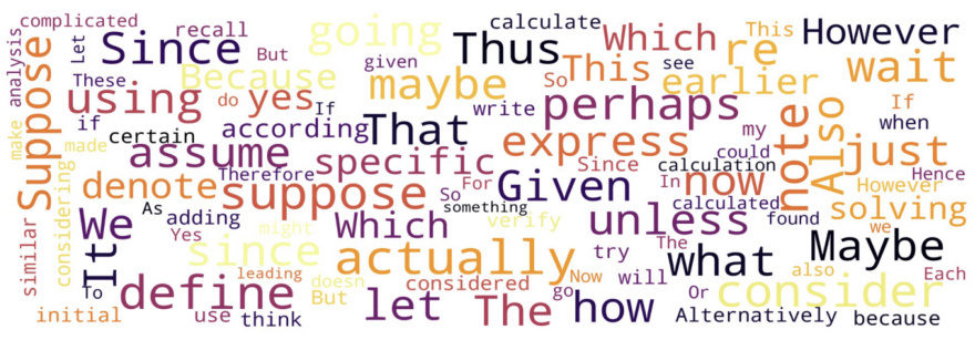
Different strategies boost the impact of RL on these tokens. Most raise the upper clipping ratio to allow more aggressive updates on them — DAPO, JustRL, Lite-PPO, MiniRL. Others limit the update on them instead. Both directions also help slow the entropy decrease of the policy.
Length normalisation and reward shaping
The original GRPO objective weights down each trajectory gradient by its length, \(\frac{1}{|y_i|}\), so that every token is weighted equally between trajectories. Whether this is right is disputed.
- For DAPO and Dr. GRPO it is an error carried over from supervised learning, biasing answers toward shorter positive trajectories or longer negative ones.
- Others argue it is a useful bias, promoting long answers and thus encouraging reasoning chains to emerge.
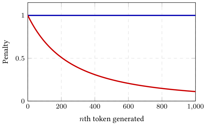
Separately, an active line of work introduces explicit length-related reward terms, motivated by the observation that reasoning models tend to over-expand their chain-of-thought even on trivial prompts. The simplest schemes apply a constant penalty on response length. Applying such a penalty too early or too strongly tends to collapse exploration and accuracy. More refined schemes, such as Cursor Composer 2, adapt the penalty to task difficulty, so the model is forced to be concise on easy prompts but can think longer when the problem warrants it.
Dynamic sampling
Some setups — DAPO, INTELLECT-3 — ensure that training prompts produce a useful learning signal. This can be done within a batch, by filtering out prompts whose rollouts are all correct or all incorrect, or over a longer horizon, by curriculum-style sampling that progressively favours harder prompts.
The reason a uniform group is worthless follows from the previous section. If every \(R_i\) is equal, then \(R_i - \operatorname{mean}(R) = 0\) for all \(i\), and the prompt contributes no gradient at all.
Sequence-level objectives
Because only one reward arrives at the very end of the episode, the MDP can be reformulated at sequence level:
\[J^{\text{GRPO,seq}}(\theta) = \mathbb{E}_{\substack{x \sim \mathcal{D} \\ \{y_i\}_{i=1}^G \sim \pi_{\theta_{\text{old}}}(\cdot|x)}} \left[ \frac{1}{G} \sum_{i=1}^G \min(s_i(\theta) \, \hat{A}_i, \operatorname{clip}(s_i(\theta), 1-\epsilon, 1+\epsilon) \, \hat{A}_i) \right]\]
Instead of each generated token being an action, the whole sequence is a single action. A trajectory is a single transition: one state \(x\), one action \(y\), one reward. The importance ratio becomes
\[s_i(\theta) = \frac{\pi_\theta(y_i \mid x)}{\pi_{\theta_{\text{old}}}(y_i \mid x)} = \prod_t \rho_{i,t}(\theta).\]
This is a valid choice but is not made as is in practice. The sequence-level ratio has variance growing multiplicatively with \(|y_i|\), which is prone to instability and makes the clipping range \([1-\epsilon, 1+\epsilon]\) hard to calibrate across rollouts of different lengths. Two responses follow.
Zheng et al. (2025) shows the token-level objective is an approximation of the sequence-level one, valid when \(\theta \approx \theta_{\text{old}}\), and argues the sequence-level form is more principled for RLVR.
Under it, the initial state distribution depends only on the dataset, so the trust region approximation \(d^{\pi_\theta} \approx d^{\pi_{\theta_{\text{old}}}}\) becomes exact rather than approximate.
GSPO optimises the sequence-level objective but replaces the ratio with a length-normalised version to mitigate the variance:
\[s_i(\theta) = \left(\frac{\pi_\theta(y_i \mid x)}{\pi_{\theta_{\text{old}}}(y_i \mid x)}\right)^{1/|y_i|}\]
Key ideas
- Whether RLVR creates new capability or better samples existing ones is unresolved.
- The gradient concentrates on the few tokens where the model was uncertain.
- Length is where reward hacking reappears, and every fix for it trades against exploration.
- A group with uniform reward gives zero advantage, so it is filtered out.
- Token-level and sequence-level objectives are the same objective under a small-drift approximation; the sequence-level form is cleaner but higher variance.
Learning outcomes
- rlvr-refinements Evaluate the practical refinements to GRPO — entropy targeting, length penalties, dynamic sampling and sequence-level objectives.
- grpo Explain how GRPO removes the critic by using a group of sampled completions as its baseline.
Concepts
- high-entropy-tokens examines how RLVR updates primarily alter high-entropy forking tokens, and the methods that adjust clipping bounds on them
- sequence-level-rl analyses sequence-level MDP formulations and length-normalised objectives like GSPO to control importance sampling variance
- rlvr discusses emerging capabilities, length penalties and reward shaping to refine reasoning behaviour under RLVR
RL infrastructure
The pseudocode of GRPO fits in fewer than 30 lines. Implementing an efficient RLVR training loop is a substantial systems engineering effort. This is the section where the on-policy/off-policy distinction from II Diving Deeper stops being theory.
The loop relies on two main components.
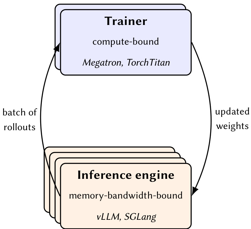
- The trainer consumes batches of experience and runs GRPO — or another algorithm — to update the policy weights.
- The inference engine collects rollouts by executing the policy in the environment. This can involve tool use, such as web requests, or code execution.
Each typically runs on multiple interconnected GPU nodes, and the two workloads are very different: training is compute-bound, inference is memory-bandwidth-bound. They use different frameworks — Megatron or TorchTitan against vLLM or SGLang — and must be orchestrated to minimise idle time on either side.
A further difficulty compounds over training. As the policy improves it generates longer rollouts: longer reasoning chains, more tool calls. Because attention costs grow quadratically in sequence length, inference becomes disproportionately more expensive as training progresses.
Three optimisations, and what they cost
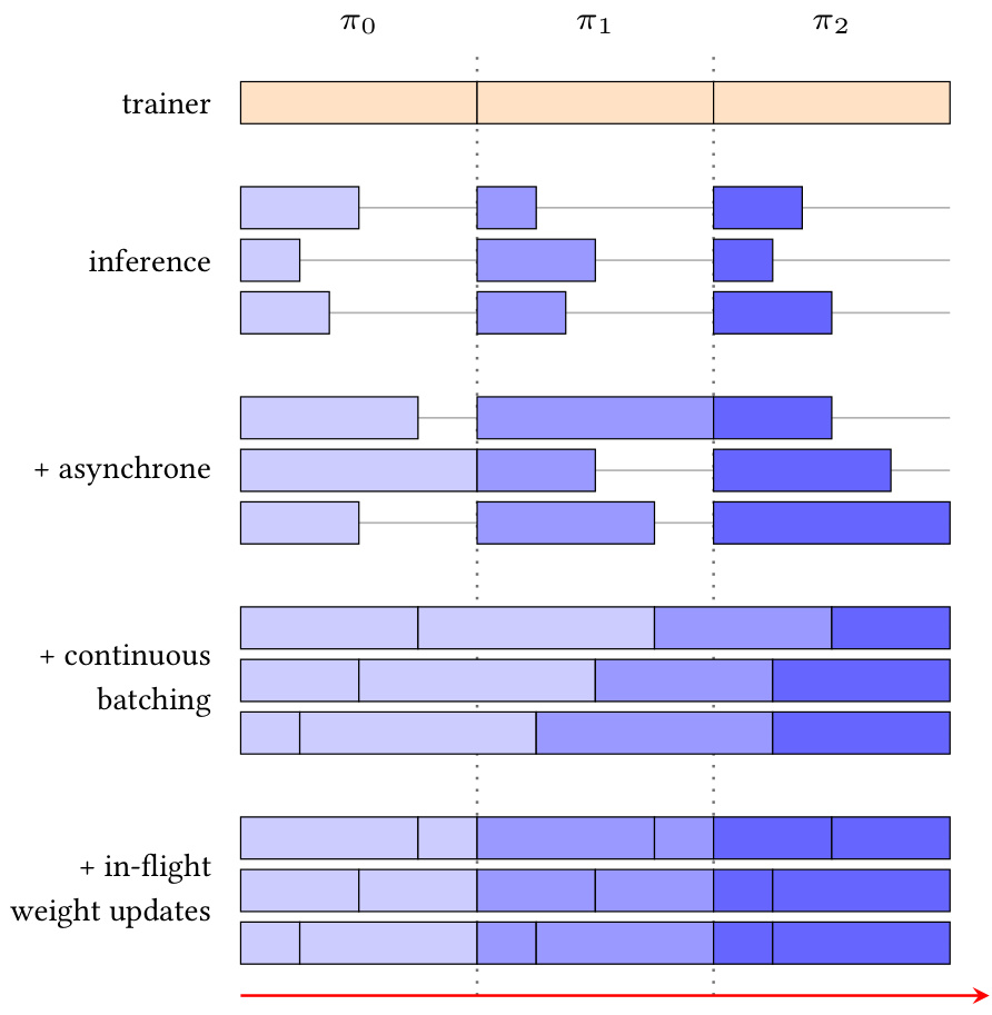
Asynchronous training and inference. The two components run in parallel without waiting for each other. After collecting a batch of rollouts, the inference engine does not wait for updated weights before starting the next batch.
The rollouts are therefore collected with an older policy, which introduces off-policyness.
Continuous batching. Rollouts in one batch differ greatly in response length and tool use, so much time is lost waiting for the longest to finish. Continuous batching repopulates a rollout slot as soon as it is free.
In-flight weight updates. The inference engine continuously polls the trainer for new weights and uses the latest policy as soon as it is available. A single rollout is then generated by several policies, which in a sense limits off-policyness.
These optimisations are a trade-off between hardware efficiency and algorithmic fidelity.
Two drifts, one ratio
A second, subtler problem is the mismatch between the training and inference engines. It is worsened by Mixture-of-Experts layers, where a slight numerical difference can route tokens to different experts, amplifying the discrepancy. The rollout policy, written \(\mu_\theta\), uses the same weights as the training policy \(\pi_\theta\) yet produces different outputs — which biases the gradient estimator.
The fix is to account for the discrepancy in a second importance sampling ratio,
\[\frac{\pi_{\theta_{\text{old}}}(y_t \mid x, y_{<t})}{\mu_{\theta_{\text{old}}}(y_t \mid x, y_{<t})},\]
leading to a global ratio
\[\rho_t(\theta) = \frac{\pi_\theta(y_t \mid x, y_{<t})}{\mu_{\theta_{\text{old}}}(y_t \mid x, y_{<t})} = \frac{\pi_\theta(y_t \mid x, y_{<t})}{\pi_{\theta_{\text{old}}}(y_t \mid x, y_{<t})} \cdot \frac{\pi_{\theta_{\text{old}}}(y_t \mid x, y_{<t})}{\mu_{\theta_{\text{old}}}(y_t \mid x, y_{<t})}.\]
The two factors correct two different things. The first corrects for having performed multiple updates and therefore drifted from the old policy. The second corrects the training-inference mismatch. The expectation is now taken under the rollout policy \(\mu_{\theta_{\text{old}}}\), and \(\rho_t(\theta)\) is what makes that legitimate.
Learning outcomes
- rl-infrastructure Describe an RLVR training system: separate trainer and inference fleets, and the importance-sampling corrections their drift demands.
Concepts
- rlvr-infrastructure details the distributed systems layout, asynchronous execution and importance sampling corrections for RLVR
- rlvr describes the practical engineering and scaling constraints of running RLVR training loops over long horizons
Blurring SFT and RL
Some methods deliberately blur the line between SFT and RL, to take the strengths of both. To see why, set the two side by side on a single axis.
- RL performs on-policy training. It learns from situations the model actually encounters, rather than from situations encountered by an expert or a teacher. This is much more robust, since the student is likely to drift from the expert’s situations at inference, and it enables grounding. But the learning signal is sparse.
- SFT provides a dense learning signal — a target on every token — but performs off-policy training.
Each has exactly what the other lacks.
On-Policy Distillation
On-Policy Distillation samples situations from a student model and uses a teacher model to provide targets on those situations. It can be viewed as a token-level version of DAgger applied in the LLM context, and it combines the advantages of on-policy training with a dense learning signal.
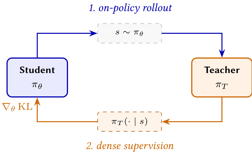
DAgger — Dataset Aggregation, Ross et al. (2011) — is the classical imitation-learning answer to covariate shift: query the expert on states the learner itself visits, not on states the expert would have visited.
Why SFT memorises
Multiple works have shown that SFT tends to induce memorisation while RL induces generalisation. DFT — Dynamic Fine-Tuning — may offer an explanation, by rewriting the SFT objective as a policy gradient objective:
\[\nabla_\theta \mathcal{J}^{\text{SFT}}(\theta) = \mathbb{E}_{x \sim \mathcal{D}, y \sim \pi_\theta(\cdot \mid x)} \left[ w(y \mid x) \, \nabla_\theta \log \pi_\theta(y \mid x) \, r(x, y) \right]\]
with
\[w(y \mid x) = \frac{1}{\pi_\theta(y \mid x)}, \qquad r(x, y) = \mathbb{I}\{y = y^*\}.\]
Read that carefully. SFT is policy gradient with a reward that is \(1\) if the model output matches the target and \(0\) otherwise — weighted by a scalar that inflates updates on low-probability targets. That weight is what biases the model toward memorising specific \((x, y^*)\) pairs instead of learning a generalisable policy.
It is tempting to describe SFT as “policy gradient with the advantage fixed at a constant”. The derivation above says otherwise: the weight is \(1/\pi_\theta(y \mid x)\), which grows without bound as the target becomes improbable under the current policy. The pathology is precisely in that dependence.
The practical reading is that SFT and RL are two settings of the same objective’s reward and weight. Once you see that, the hybrids stop looking like tricks. On-Policy Distillation fixes the distribution the states are drawn from; DFT fixes the weight.
Learning outcomes
- sft-rl-continuum Explain how SFT and RL relate as objectives, and describe the hybrid methods that sit between them.
- post-training-regimes Distinguish SFT, RLHF and RLVR as post-training regimes, and say what each optimises and where each fails.
Concepts
- on-policy-distillation introduces On-Policy Distillation as a bridge combining on-policy sampling with dense teacher token supervision
- rlvr compares SFT’s tendency to memorise against RL’s capability to induce generalisable reasoning
AlphaGo Zero: search as improvement
We now change domain entirely. AlphaGo Zero can be seen as a form of policy iteration coupled with a model-based approach. During training it alternates between two phases.
- Improvement. Instead of acting according to the current policy, act according to an improved version of it. The improvement is done through planning — searching in the environment — and so leverages the known dynamics, which for Go are the hard-coded rules of the game.
- Evaluation. Fit the current policy and value function to the experience collected using the improved policy.
Neural networks represent both the policy \(\pi_\theta\) and the value function \(V_\phi\). A particularly striking aspect is that training is done through self-play: the agent plays against another version of itself. No human data is needed, and the agent learns from scratch.
The improvement step
The improvement step happens each time the agent has to pick an action, rather than globally at the end of an episode as in traditional policy iteration.
Consider a state \(s_0\) the agent must act on. The goal is an action \(a\) chosen according to an improved version of \(\pi_\theta\). This is done by traversing the Bellman backup diagram starting from \(s_0\). Rather than traverse it exhaustively — impossible in Go — AlphaGo Zero grows a partial tree, concentrating computation on the regions that look promising under the current \(\pi_\theta\) and \(V_\phi\).
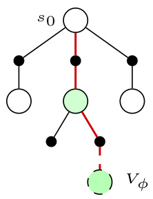
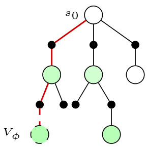
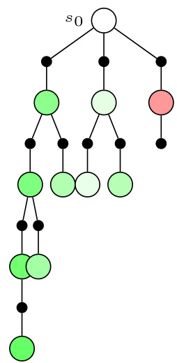
Each traversal, shown in red, follows a selection rule trading off exploration and exploitation. It expands the tree by one node and backs up the statistics of the path it followed, starting from the bootstrap \(V_\phi(\text{leaf})\). The most promising lines of play are therefore the most densely explored. The book describes this as a modified version of an MCTS rollout.
After a fixed budget of traversals, the visit counts at the root concentrate on the most promising actions and define an improved policy at \(s_0\), from which the agent samples its action. We will write that improved policy \(\mu\).
What the search is doing
The improvement step can be understood as approximating the optimality Bellman operator
\[V_\phi(s_0) \leftarrow \max_a \mathbb{E}\left[ r(s_0, a, s') + \gamma V_\phi(s') \right],\]
using the tree, and using the policy as a prior to focus the search and make it tractable.
More intuitively: think of the base policy \(\pi_\theta\) as an intuition policy, and the search as a thinking process that mentally unrolls and simulates possible futures.
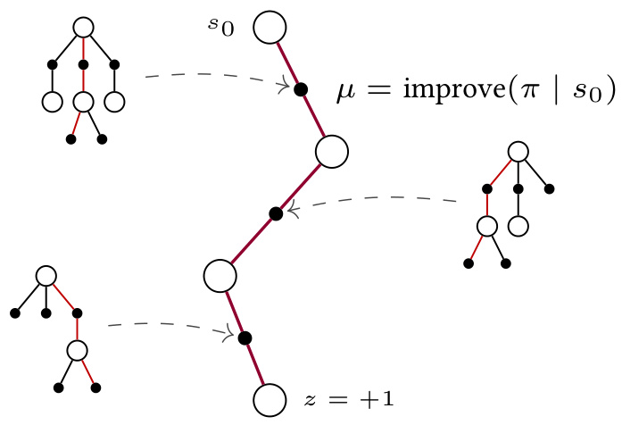
The prior is what makes this tractable. Go has roughly 250 legal moves per position; an unguided tree search over that branching factor is hopeless. \(\pi_\theta\) tells the search which handful to bother with.
Learning outcomes
- alphago-zero-loop Explain AlphaGo Zero as policy iteration where MCTS is the improvement operator and self-play rollouts are the evaluation.
Concepts
- alphago-zero-policy-iteration details the MCTS partial tree traversal and root visit distribution that represent the improved policy
AlphaGo Zero: evaluation and distillation
Once experience has been collected by acting according to the improved policy, and rewards \(z\) collected, the evaluation phase takes place. Two networks are fitted, with two different kinds of target.
The value function is fit to evaluate the improved policy, using Monte Carlo evaluation:
\[\mathcal{L}_V(\phi) = \sum_s (V_\phi(s) - z)^2.\]
This is the Monte Carlo return estimator from II Diving Deeper, unchanged. The game outcome is the return, and there is no bootstrapping in the target.
The base policy is trained using behaviour cloning — that is, SFT — to reproduce the improved policy:
\[\mathcal{L}_\pi(\theta) = -\sum_s \sum_a \mu(a \mid s) \log \pi_\theta(a \mid s).\]
Cross-entropy against the search’s own action distribution. The network is being taught to guess, in one forward pass, what the search worked out slowly.
System 1 and System 2
The book gives this loop its name. The base policy \(\pi\) can be seen as the fast, intuitive System 1, and the search-improved policy \(\mu\) as the slow, deliberate System 2. The evaluation phase distils System 2 back into System 1.
That framing explains why the loop bootstraps rather than stalling. Recall from the previous section that the search uses \(\pi_\theta\) as its prior and \(V_\phi\) as its bootstrap at the leaves. So:
- A better prior focuses the search on better lines, so the same traversal budget produces a stronger \(\mu\).
- A stronger \(\mu\) is a better cross-entropy target, so the next \(\pi_\theta\) is better still.
- A better \(V_\phi\) makes the leaf evaluations more accurate, which improves the search independently.
The network never has to be told what a good move is. It only has to be told what its own search decided, and the search is reliably better than the network that guided it.
Notice that the value head is fit against the outcome \(z\) and not against \(\mu\). If both heads were fit against the search, nothing in the loop would touch the ground. The game result is the only external signal in the entire system, and it enters here.
Key ideas
- Evaluation fits \(V_\phi\) to the realised outcome \(z\) by regression, and \(\pi_\theta\) to the search policy \(\mu\) by cross-entropy.
- Distillation compresses deliberate search into a single forward pass.
- The improved prior feeds the next search, which produces better targets — the loop is self-reinforcing without human data.
Learning outcomes
- alphago-zero-loop Explain AlphaGo Zero as policy iteration where MCTS is the improvement operator and self-play rollouts are the evaluation.
Concepts
- alphago-zero-policy-iteration describes training the neural value and policy networks using self-play outcomes and MCTS visit distributions
Self-play dynamics
Go is a two-player game, so the agent needs an opponent to play against in order to collect experience. AlphaGo Zero uses self-play: it plays against another version of itself.
The immediate benefit is practical. No human data is required at all. A second benefit follows from the arrangement rather than from any design effort — the agent always faces an opponent of its own level, providing some sort of curriculum learning. Difficulty tracks competence automatically, because difficulty is competence here.
Why it does not degenerate
Self-play sounds unstable. The opponent changes every time the agent improves, and in general a moving opponent is a moving target. The book gives two specific reasons that this arrangement does not degenerate into a suboptimal strategy.
The targets are grounded rather than self-referential. The regression is done toward a search-improved version of the policy, and toward real game outcomes, rather than toward the network’s own predictions.
This is the point of the previous section. \(V_\phi\) chases \(z\), a fact about the world. Nothing in the loop is allowed to chase only itself.
The two-player zero-sum perfect-information structure ensures any exploitable weakness on one side is punished by the symmetric opponent. There is no mutually agreeable strategy for two copies of a player to settle into, because one player’s gain is exactly the other’s loss.
Together these drive training toward the unique minimax equilibrium of the game.
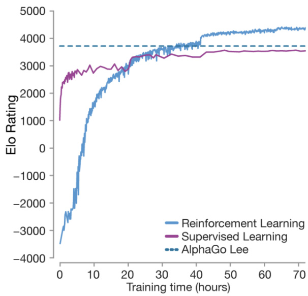
Both reasons above appeal to structure: grounded targets, and two-player zero-sum perfect information. Self-play in a general-sum or cooperative setting has neither guarantee, and collusive or degenerate equilibria are exactly what it can find. Do not carry the convergence claim across without carrying the conditions.
Learning outcomes
- self-play-and-test-time-compute Explain why zero-sum self-play converges rather than collapses, and what a task needs before AlphaZero transfers to it.
Concepts
- alphago-zero-policy-iteration explains how two-player zero-sum self-play converges to a minimax equilibrium without human data
Test-time compute and transfer
At test time, AlphaGo Zero acts as it does in training. It does not use its policy directly to pick actions; it performs the MCTS-like improvement step described above. This can be seen as a form of test-time compute.
The size of the effect is worth stating precisely. Using the base policy — the “Raw Network” — is far less effective than using the search-improved policy. The raw network loses against its improved version more than \(99.99\%\) of the time.
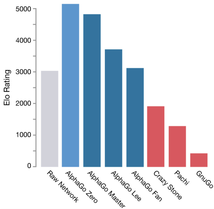
That is the same network, with the same weights, in both columns. The entire difference is computation spent at inference. It is a dial available after training is finished, and it is the closest thing in this unit to a free improvement.
What a task must supply
The AlphaGo Zero recipe, generalised under the name AlphaZero, is very strong. But it relies on a specific setup. The book lists three requirements.
- Known or learnable dynamics. You must be able to simulate the consequence of an action without taking it.
- A tractable action space. The search has to branch over the legal actions, so their number must be manageable.
- Cheap simulated rollouts. A budget of traversals per move is only affordable if each traversal is nearly free.
Where these conditions hold, the recipe transfers remarkably well — AlphaTensor, AlphaDev, AlphaProof, Aristotle. Where they do not, it is far from a plug-and-play recipe. There has been a strong push to apply it to LLM training, with no clear public success so far.
Compare the two halves of this unit against the three conditions. Text generation has no fast exact model of “what happens next” in any useful sense, and its action space is the whole vocabulary at every step. RLVR sidesteps the problem: rather than searching over futures, it samples \(G\) complete futures and scores them. GRPO is what remains of the idea when the search is unaffordable.
Learning outcomes
- self-play-and-test-time-compute Explain why zero-sum self-play converges rather than collapses, and what a task needs before AlphaZero transfers to it.
- alphago-zero-loop Explain AlphaGo Zero as policy iteration where MCTS is the improvement operator and self-play rollouts are the evaluation.
Concepts
- test-time-compute illustrates how AlphaGo Zero’s test-time MCTS execution constitutes test-time compute that outperforms the raw base network
- alphago-zero-policy-iteration discusses the domain conditions required for AlphaZero transfer, and the difficulty of applying it to LLMs
Recurring patterns across RL
The book closes by naming a few patterns that surfaced more than once across its chapters. They are the most portable thing in this module, because they outlast any particular algorithm.
Credit assignment. Every RL algorithm provides a way of attributing credit through time: bootstrapping in TD, returns in MC, the policy gradient theorem in policy optimisation.
The same problem appears for a delayed reward in a control task and for a single verifier score arriving after a thousand tokens.
Bias and variance. They appear in the choice between MC and TD, in the depth of \(n\)-step returns, in the \(\lambda\) of GAE, in the importance ratio of PPO, and in the group baseline of GRPO. Every estimator in RL faces this trade-off.
The data distribution moves. This is what fundamentally separates RL from supervised learning. The agent generates its own training data, and any update changes which data it will see next. Design choices like trust regions manage this drift.
On-policy versus off-policy. How stale is the data relative to the current policy? Q-learning tolerates arbitrary staleness by decoupling the behaviour policy from the target policy, while PPO and GRPO use trust regions.
This one has practical limitations in modern RL infrastructures — precisely the asynchronous rollouts and engine mismatch of §RL infrastructure.
The edges of the map
Many active areas of RL were left out of the book, and therefore out of this module. It is worth knowing their names.
- Offline RL — learning a policy from a fixed dataset without further interaction: CQL, IQL, behaviour cloning baselines.
- Deterministic policy gradients — DDPG, TD3, SAC, and the off-policy actor-critic line behind modern robotics.
- Model-based RL — Dreamer, MuZero, PlaNet, and learned world models for planning.
- Exploration — multi-armed bandits, intrinsic motivation such as RND and ICM, Thompson sampling, posterior sampling.
- Multi-agent RL — general-sum games, equilibrium concepts, opponent modelling.
- Inverse RL — recovering rewards from demonstrations.
- Hierarchical RL — options, sub-goals, temporal abstraction.
For going further, the book recommends Sutton and Barto’s Reinforcement Learning: An Introduction for the classical theory, Spinning Up in Deep RL for clean PyTorch implementations, CleanRL and PufferLib for fast iteration, and The RLHF Book for post-training of language models.
Learning outcomes
- unifying-patterns Identify the recurring patterns — credit assignment, bias-variance, moving distributions and data staleness — in any RL algorithm you meet.
- rl-infrastructure Describe an RLVR training system: separate trainer and inference fleets, and the importance-sampling corrections their drift demands.
Closing the module
This is the last unit of Reinforcement Learning, and the last unit of the curriculum. You can now:
- Distinguish SFT, RLHF and RLVR, and explain why a deterministic verifier resists the reward hacking a learned reward model invites.
- Write LLM generation as an MDP with deterministic transitions and a sparse terminal reward, regularised by a KL penalty against a reference policy.
- Explain GRPO as PPO with the critic replaced by the group mean, and evaluate the refinements layered on it.
- Describe an RLVR training system, and apply the two importance sampling ratios that correct asynchronous drift and engine mismatch.
- Explain AlphaGo Zero as policy iteration with search in the improvement slot, distilled back into the network.
- Say why zero-sum self-play converges, and what a task must supply before AlphaZero transfers to it.
- Read a new RL algorithm through four lenses: distribution shift, credit assignment, bias-variance, and data staleness.
Look back at the arc. I Foundations gave you the vocabulary — reward, return, policy, value, the MDP, and the taxonomy that organises the field. II Diving Deeper turned that vocabulary into algorithms that learn, from a tabular Bellman backup to PPO’s clipped surrogate. This unit ran those algorithms on a thousand-GPU cluster and on a Go board, and found the same four concerns waiting in both.
That is the durable result of the module. The algorithms in this unit are recent and will be superseded; several of the debates in §Beyond GRPO were unresolved at the time the book was written. The four patterns will not be superseded. When the next method arrives, ask it how it assigns credit, where it sits on the bias-variance spectrum, how it handles its own moving data distribution, and what it pays for stale data. Those four questions will get you most of the way through any paper in this field.
Learning outcomes
- post-training-regimes Distinguish SFT, RLHF and RLVR as post-training regimes, and say what each optimises and where each fails.
- llm-generation-as-mdp Formalise token generation as an MDP and identify the state, action, transition and reward of an RLVR run.
- grpo Explain how GRPO removes the critic by using a group of sampled completions as its baseline.
- rlvr-refinements Evaluate the practical refinements to GRPO — entropy targeting, length penalties, dynamic sampling and sequence-level objectives.
- rl-infrastructure Describe an RLVR training system: separate trainer and inference fleets, and the importance-sampling corrections their drift demands.
- sft-rl-continuum Explain how SFT and RL relate as objectives, and describe the hybrid methods that sit between them.
- alphago-zero-loop Explain AlphaGo Zero as policy iteration where MCTS is the improvement operator and self-play rollouts are the evaluation.
- self-play-and-test-time-compute Explain why zero-sum self-play converges rather than collapses, and what a task needs before AlphaZero transfers to it.
- unifying-patterns Identify the recurring patterns — credit assignment, bias-variance, moving distributions and data staleness — in any RL algorithm you meet.
References
- The Little Book of Reinforcement Learning, Alexandre Torres Leguet, 2026 — Link — Page 112-154