Feature Pyramid Networks for Object Detection

A technical walkthrough of Feature Pyramid Networks (FPN), the architecture that builds multi-scale feature representations with strong semantics at all levels, enabling state-of-the-art object detection from a single input image scale.

The Problem: Multi-Scale Object Detection

Recognizing objects at vastly different scales is a fundamental challenge in computer vision. A pedestrian far away might occupy 32x32 pixels, while a nearby car fills 512x512 pixels. A robust detector must handle both.

The classical solution is the featurized image pyramid: resize the input image to multiple scales, extract features at each scale independently, and run detection on every level. This approach is scale-invariant by construction — an object’s scale change is offset by shifting its level in the pyramid. Detectors like DPM required dense scale sampling (10 scales per octave) and relied heavily on this representation.

However, featurized image pyramids have a critical limitation: inference time increases by roughly 4x because the entire feature extraction pipeline must be repeated for each scale. Training end-to-end on image pyramids is infeasible in terms of memory, so pyramids are typically used only at test time, creating an inconsistency between training and testing.

Modern deep learning detectors like Fast R-CNN and Faster R-CNN took a different path: they operate on a single-scale feature map from a deep ConvNet. ConvNets are robust to scale variation thanks to their learned representations, and single-scale inference offers a good speed-accuracy trade-off. But this approach sacrifices multi-scale detection, especially for small objects.

The question that FPN addresses is: can we build a feature pyramid with strong semantics at all scales, from a single input image, at marginal extra cost?

Prior Approaches and Their Limitations

Before FPN, there were four main strategies for multi-scale feature extraction. Each has significant drawbacks.

import matplotlib.pyplot as plt
import matplotlib.patches as patches
import numpy as np

fig, axes = plt.subplots(1, 4, figsize=(16, 5))

def draw_pyramid(ax, title, subtitle, draw_func):
    ax.set_xlim(0, 10)
    ax.set_ylim(0, 10)
    ax.axis('off')
    ax.set_title(title, fontsize=10, fontweight='bold', pad=8)
    ax.text(5, 0.2, subtitle, ha='center', va='bottom', fontsize=7,
            style='italic', color='#555555')
    draw_func(ax)

# (a) Featurized image pyramid
def draw_a(ax):
    sizes = [(3.5, 3.5), (2.8, 2.8), (2.0, 2.0), (1.3, 1.3)]
    ys = [1.5, 3.5, 5.5, 7.2]
    for i, ((w, h), y) in enumerate(zip(sizes, ys)):
        x = 5 - w/2
        # Image (light blue)
        ax.add_patch(patches.FancyBboxPatch((x-0.8, y), w, h, boxstyle='round,pad=0.05',
                     facecolor='#BBDEFB', edgecolor='#1565C0', linewidth=1.5))
        ax.text(x-0.8+w/2, y+h/2, f'img', ha='center', va='center', fontsize=7, color='#1565C0')
        # Feature (darker blue)
        ax.add_patch(patches.FancyBboxPatch((x+0.8, y), w, h, boxstyle='round,pad=0.05',
                     facecolor='#1565C0', edgecolor='#0D47A1', linewidth=1.5))
        ax.text(x+0.8+w/2, y+h/2, f'feat', ha='center', va='center', fontsize=7, color='white')
        # Arrow
        ax.annotate('', xy=(x+0.8, y+h/2), xytext=(x-0.8+w, y+h/2),
                    arrowprops=dict(arrowstyle='->', color='gray', lw=1))
        # Predict
        ax.annotate('predict', xy=(x+0.8+w+0.1, y+h/2), fontsize=6, color='#2E7D32',
                    fontweight='bold', va='center')

draw_pyramid(axes[0], '(a) Featurized\nImage Pyramid',
             'Slow (~4x cost)', draw_a)

# (b) Single feature map
def draw_b(ax):
    # Single large image
    ax.add_patch(patches.FancyBboxPatch((2, 1.5), 3.5, 3.5, boxstyle='round,pad=0.05',
                 facecolor='#BBDEFB', edgecolor='#1565C0', linewidth=1.5))
    ax.text(3.75, 3.25, 'image', ha='center', va='center', fontsize=8, color='#1565C0')
    # Arrow down to single feature
    ax.annotate('', xy=(5, 6.5), xytext=(5, 5.2),
                arrowprops=dict(arrowstyle='->', color='gray', lw=1.5))
    # Single feature map (small, dark)
    ax.add_patch(patches.FancyBboxPatch((3.8, 6.5), 1.5, 1.5, boxstyle='round,pad=0.05',
                 facecolor='#1565C0', edgecolor='#0D47A1', linewidth=2.5))
    ax.text(4.55, 7.25, 'feat', ha='center', va='center', fontsize=8, color='white')
    ax.annotate('predict', xy=(5.5, 7.25), fontsize=7, color='#2E7D32',
                fontweight='bold', va='center')

draw_pyramid(axes[1], '(b) Single\nFeature Map',
             'Fast but misses multi-scale', draw_b)

# (c) Pyramidal feature hierarchy (SSD-style)
def draw_c(ax):
    sizes = [3.0, 2.2, 1.5, 1.0]
    ys = [1.5, 3.5, 5.5, 7.5]
    blues = ['#BBDEFB', '#64B5F6', '#1E88E5', '#0D47A1']
    for i, (s, y, c) in enumerate(zip(sizes, ys, blues)):
        x = 5 - s/2
        lw = 1.0 + i * 0.5
        ax.add_patch(patches.FancyBboxPatch((x, y), s, s*0.7, boxstyle='round,pad=0.05',
                     facecolor=c, edgecolor='#0D47A1', linewidth=lw))
        if i > 0:
            ax.annotate('', xy=(5, y), xytext=(5, ys[i-1]+sizes[i-1]*0.7),
                        arrowprops=dict(arrowstyle='->', color='gray', lw=1))
        # Only predict from higher layers (SSD skips early ones)
        if i >= 1:
            ax.annotate('predict', xy=(x+s+0.2, y+s*0.35), fontsize=6, color='#2E7D32',
                        fontweight='bold', va='center')

draw_pyramid(axes[2], '(c) Pyramidal Feature\nHierarchy (SSD)',
             'Weak semantics at low levels', draw_c)

# (d) FPN
def draw_d(ax):
    sizes = [3.0, 2.2, 1.5, 1.0]
    ys = [1.5, 3.5, 5.5, 7.5]
    # Bottom-up (left)
    blues = ['#BBDEFB', '#64B5F6', '#1E88E5', '#0D47A1']
    for i, (s, y, c) in enumerate(zip(sizes, ys, blues)):
        x = 3 - s/2
        lw = 1.0 + i * 0.5
        ax.add_patch(patches.FancyBboxPatch((x, y), s, s*0.6, boxstyle='round,pad=0.05',
                     facecolor=c, edgecolor='#0D47A1', linewidth=lw))
        if i > 0:
            ax.annotate('', xy=(3, y), xytext=(3, ys[i-1]+sizes[i-1]*0.6),
                        arrowprops=dict(arrowstyle='->', color='gray', lw=1))
    # Top-down + lateral (right)
    for i, (s, y) in enumerate(zip(sizes, ys)):
        x = 7 - s/2
        lw = 2.0
        ax.add_patch(patches.FancyBboxPatch((x, y), s, s*0.6, boxstyle='round,pad=0.05',
                     facecolor='#0D47A1', edgecolor='#01579B', linewidth=lw))
        # Lateral connection
        left_x = 3 + sizes[i]/2
        right_x = 7 - sizes[i]/2
        ax.annotate('', xy=(right_x, y+s*0.3), xytext=(left_x, y+s*0.3),
                    arrowprops=dict(arrowstyle='->', color='#E53935', lw=1.2, linestyle='--'))
        # Top-down
        if i < len(sizes)-1:
            ax.annotate('', xy=(7, ys[i]+sizes[i]*0.6), xytext=(7, ys[i+1]),
                        arrowprops=dict(arrowstyle='->', color='#FF9800', lw=1.2))
        # Predict from every level
        ax.annotate('predict', xy=(7+sizes[i]/2+0.1, y+s*0.3), fontsize=6,
                    color='#2E7D32', fontweight='bold', va='center')

draw_pyramid(axes[3], '(d) Feature Pyramid\nNetwork (FPN)',
             'Fast + strong semantics at all levels', draw_d)

plt.suptitle('Four Approaches to Multi-Scale Feature Extraction',
             fontsize=14, fontweight='bold', y=1.02)
plt.tight_layout()
plt.show()

The four approaches differ in how they trade off speed, semantic strength, and multi-scale coverage:

Approach	Speed	Semantics	Multi-Scale	Key Limitation
(a) Featurized image pyramid	Slow (~4x)	Strong at all levels	Yes	Computationally expensive; train/test inconsistency
(b) Single feature map	Fast	Strong (one level)	No	Misses small/large objects
(c) Pyramidal hierarchy (SSD)	Fast	Weak at low levels	Partial	Skips high-res layers; poor for small objects
(d) Top-down + skip (U-Net)	Fast	Strong at finest level	Partial	Predictions only at finest level; still needs image pyramids

ImportantThe Gap That FPN Fills

SSD-style pyramidal hierarchies reuse the ConvNet’s natural multi-scale feature maps, but lower layers have weak semantics and SSD deliberately skips early (high-resolution) layers, missing features critical for detecting small objects. U-Net-style architectures enrich features via top-down pathways, but make predictions only at the finest level, not independently at each scale. FPN combines the best of both: strong semantics at every pyramid level with independent predictions at each scale.

Core Contribution: The FPN Architecture

Feature Pyramid Networks build a feature pyramid with strong semantics at all scales from a single input image. The architecture consists of three components:

1. Bottom-up pathway — the standard feedforward ConvNet
2. Top-down pathway — upsampling from coarse to fine resolution
3. Lateral connections — merging bottom-up and top-down features

Bottom-Up Pathway

The bottom-up pathway is simply the forward pass of the backbone ConvNet (e.g., ResNet). It computes a feature hierarchy at several scales with a scaling step of 2. For ResNets, FPN uses the output of each stage’s last residual block:

• \(C_2\) from conv2 — stride 4
• \(C_3\) from conv3 — stride 8
• \(C_4\) from conv4 — stride 16
• \(C_5\) from conv5 — stride 32

Conv1 is excluded due to its large memory footprint.

Top-Down Pathway and Lateral Connections

The top-down pathway generates higher-resolution features by upsampling spatially coarser but semantically stronger feature maps from higher pyramid levels. These are then enhanced with bottom-up features via lateral connections.

The building block works as follows:

1. Take a coarser feature map and upsample by 2x (nearest neighbor)
2. Take the corresponding bottom-up map and apply a 1x1 convolution to reduce its channels to \(d = 256\)
3. Element-wise addition merges the two maps
4. A final 3x3 convolution reduces aliasing from upsampling

The iteration starts by applying a 1x1 conv to \(C_5\) to produce the coarsest pyramid level, then proceeds downward. The output is \(\{P_2, P_3, P_4, P_5\}\), corresponding to \(\{C_2, C_3, C_4, C_5\}\) with the same spatial sizes but all having \(d = 256\) channels.

import matplotlib.pyplot as plt
import matplotlib.patches as patches
import numpy as np

fig, ax = plt.subplots(figsize=(14, 8))
ax.set_xlim(0, 14)
ax.set_ylim(0, 10)
ax.axis('off')
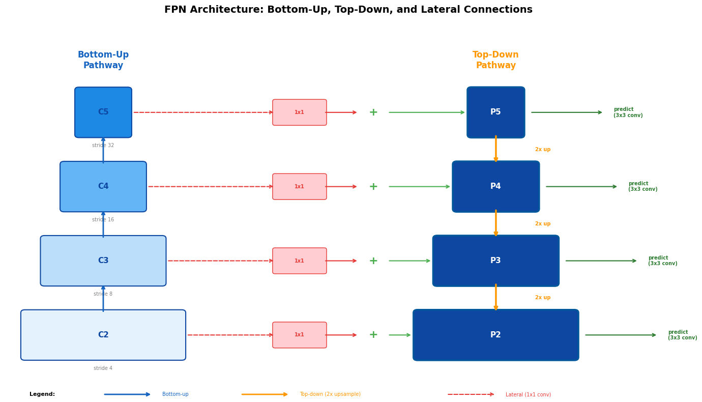
ax.set_title('FPN Architecture: Bottom-Up, Top-Down, and Lateral Connections',
             fontsize=14, fontweight='bold', pad=15)

# Bottom-up pathway (left side)
bu_x = 2.0
bu_levels = [
    ('C2', 3.2, 1.0, '#E3F2FD', 'stride 4'),
    ('C3', 2.4, 3.0, '#BBDEFB', 'stride 8'),
    ('C4', 1.6, 5.0, '#64B5F6', 'stride 16'),
    ('C5', 1.0, 7.0, '#1E88E5', 'stride 32'),
]

# Top-down pathway (right side)
td_x = 10.0
td_levels = [
    ('P2', 3.2, 1.0, '#0D47A1'),
    ('P3', 2.4, 3.0, '#0D47A1'),
    ('P4', 1.6, 5.0, '#0D47A1'),
    ('P5', 1.0, 7.0, '#0D47A1'),
]

# Draw bottom-up blocks
for name, w, y, color, stride in bu_levels:
    x = bu_x - w/2
    ax.add_patch(patches.FancyBboxPatch((x, y), w, 1.2, boxstyle='round,pad=0.08',
                 facecolor=color, edgecolor='#0D47A1', linewidth=1.5))
    ax.text(bu_x, y+0.6, f'{name}', ha='center', va='center', fontsize=11,
            fontweight='bold', color='#0D47A1')
    ax.text(bu_x, y-0.3, stride, ha='center', va='center', fontsize=7, color='gray')

# Bottom-up arrows
for i in range(len(bu_levels)-1):
    ax.annotate('', xy=(bu_x, bu_levels[i+1][2]), xytext=(bu_x, bu_levels[i][2]+1.2),
                arrowprops=dict(arrowstyle='->', color='#1565C0', lw=2))

ax.text(bu_x, 9.0, 'Bottom-Up\nPathway', ha='center', va='center', fontsize=12,
        fontweight='bold', color='#1565C0')

# Draw top-down blocks
for name, w, y, color in td_levels:
    x = td_x - w/2
    ax.add_patch(patches.FancyBboxPatch((x, y), w, 1.2, boxstyle='round,pad=0.08',
                 facecolor=color, edgecolor='#01579B', linewidth=2.5))
    ax.text(td_x, y+0.6, f'{name}', ha='center', va='center', fontsize=11,
            fontweight='bold', color='white')

# Top-down arrows (downward: P5 -> P4 -> P3 -> P2)
for i in range(len(td_levels)-1, 0, -1):
    ax.annotate('', xy=(td_x, td_levels[i-1][2]+1.2), xytext=(td_x, td_levels[i][2]),
                arrowprops=dict(arrowstyle='->', color='#FF9800', lw=2.5))
    # Label the 2x upsample
    mid_y = (td_levels[i][2] + td_levels[i-1][2]+1.2) / 2
    ax.text(td_x + 0.8, mid_y, '2x up', fontsize=7, color='#FF9800',
            fontweight='bold', va='center')

ax.text(td_x, 9.0, 'Top-Down\nPathway', ha='center', va='center', fontsize=12,
        fontweight='bold', color='#FF9800')

# Lateral connections
mid_x = 6.0
for i in range(len(bu_levels)):
    bu_name, bu_w, bu_y, _, _ = bu_levels[i]
    td_name, td_w, td_y, _ = td_levels[i]
    y_mid = bu_y + 0.6
    # Arrow from bottom-up to middle (1x1 conv)
    ax.annotate('', xy=(mid_x - 0.5, y_mid), xytext=(bu_x + bu_w/2 + 0.1, y_mid),
                arrowprops=dict(arrowstyle='->', color='#E53935', lw=1.5, linestyle='--'))
    # 1x1 conv box
    ax.add_patch(patches.FancyBboxPatch((mid_x - 0.5, y_mid - 0.3), 1.0, 0.6,
                 boxstyle='round,pad=0.05', facecolor='#FFCDD2', edgecolor='#E53935', linewidth=1))
    ax.text(mid_x, y_mid, '1x1', ha='center', va='center', fontsize=7,
            fontweight='bold', color='#E53935')
    # Addition symbol
    add_x = mid_x + 1.5
    ax.text(add_x, y_mid, '+', ha='center', va='center', fontsize=16,
            fontweight='bold', color='#4CAF50')
    # Arrow from 1x1 to addition
    ax.annotate('', xy=(add_x - 0.3, y_mid), xytext=(mid_x + 0.5, y_mid),
                arrowprops=dict(arrowstyle='->', color='#E53935', lw=1.5))
    # Arrow from addition to top-down block
    ax.annotate('', xy=(td_x - td_w/2 - 0.1, y_mid), xytext=(add_x + 0.3, y_mid),
                arrowprops=dict(arrowstyle='->', color='#4CAF50', lw=1.5))

# Predict arrows from each P level
for name, w, y, color in td_levels:
    pred_x = td_x + w/2 + 0.2
    ax.annotate('', xy=(pred_x + 1.5, y+0.6), xytext=(pred_x, y+0.6),
                arrowprops=dict(arrowstyle='->', color='#2E7D32', lw=1.5))
    ax.text(pred_x + 1.7, y+0.6, 'predict\n(3x3 conv)', ha='left', va='center',
            fontsize=7, color='#2E7D32', fontweight='bold')

# Legend
legend_y = 0.0
ax.text(0.5, legend_y, 'Legend:', fontsize=8, fontweight='bold', va='center')
ax.annotate('', xy=(3.0, legend_y), xytext=(2.0, legend_y),
            arrowprops=dict(arrowstyle='->', color='#1565C0', lw=2))
ax.text(3.2, legend_y, 'Bottom-up', fontsize=7, va='center', color='#1565C0')
ax.annotate('', xy=(5.8, legend_y), xytext=(4.8, legend_y),
            arrowprops=dict(arrowstyle='->', color='#FF9800', lw=2))
ax.text(6.0, legend_y, 'Top-down (2x upsample)', fontsize=7, va='center', color='#FF9800')
ax.annotate('', xy=(10.0, legend_y), xytext=(9.0, legend_y),
            arrowprops=dict(arrowstyle='->', color='#E53935', lw=1.5, linestyle='--'))
ax.text(10.2, legend_y, 'Lateral (1x1 conv)', fontsize=7, va='center', color='#E53935')

plt.tight_layout()
plt.show()

NoteDesign Principles

Simplicity is central to FPN’s design. The extra convolutional layers use no non-linearities (empirically found to have minor impact). All pyramid levels share \(d = 256\) channels. The authors experimented with more sophisticated connection blocks (e.g., multi-layer residual blocks) and observed only marginally better results. The simple design is robust to many architectural choices.

Application to RPN (Region Proposal Networks)

The original RPN evaluates a small subnetwork (a 3x3 conv followed by two sibling 1x1 convs for classification and regression) on top of a single-scale convolutional feature map. To handle objects of different sizes, it uses multi-scale anchors (multiple sizes and aspect ratios) at each spatial position.

FPN replaces the single-scale feature map with the entire feature pyramid. The key adaptations are:

1. Single-scale anchors per level: Since the pyramid already covers multiple scales, each level needs only one anchor scale. The anchors have areas of \(\{32^2, 64^2, 128^2, 256^2, 512^2\}\) pixels on \(\{P_2, P_3, P_4, P_5, P_6\}\) respectively.
2. Three aspect ratios (\(\{1{:}2, 1{:}1, 2{:}1\}\)) at each level, for a total of 15 anchors over the pyramid.
3. Shared head across all pyramid levels — the same 3x3 conv + two 1x1 conv network is applied at every level. This works because all levels share similar semantic content (analogous to applying a common classifier across scales in an image pyramid).
4. \(P_6\) is added as a stride-2 subsampling of \(P_5\) to cover the largest anchor scale of \(512^2\). It is used only for RPN, not for Fast R-CNN.

RPN Results

The impact of FPN on region proposals is dramatic, particularly for small objects.

import matplotlib.pyplot as plt
import numpy as np

# Table 1 data from the paper
labels = [
    '(a) Baseline C4',
    '(b) Baseline C5',
    '(c) FPN',
    '(d) Bottom-up only',
    '(e) Top-down\nw/o lateral',
    '(f) Only P2',
]
AR_1k = [48.3, 44.9, 56.3, 49.5, 46.1, 51.3]
AR_1k_s = [32.0, 25.3, 44.9, 30.5, 26.5, 35.1]
AR_1k_m = [58.7, 55.5, 63.4, 59.9, 57.4, 59.7]
AR_1k_l = [62.2, 64.2, 66.2, 68.0, 64.7, 67.6]

x = np.arange(len(labels))
width = 0.2

fig, ax = plt.subplots(figsize=(12, 6))

colors = ['#1565C0', '#43A047', '#F57C00', '#8E24AA']
bars1 = ax.bar(x - 1.5*width, AR_1k, width, label='AR$^{1k}$ (all)', color=colors[0], edgecolor='white')
bars2 = ax.bar(x - 0.5*width, AR_1k_s, width, label='AR$^{1k}_s$ (small)', color=colors[1], edgecolor='white')
bars3 = ax.bar(x + 0.5*width, AR_1k_m, width, label='AR$^{1k}_m$ (medium)', color=colors[2], edgecolor='white')
bars4 = ax.bar(x + 1.5*width, AR_1k_l, width, label='AR$^{1k}_l$ (large)', color=colors[3], edgecolor='white')

# Add value labels on AR_1k bars
for bar, val in zip(bars1, AR_1k):
    ax.text(bar.get_x() + bar.get_width()/2, bar.get_height() + 0.5,
            f'{val}', ha='center', va='bottom', fontsize=8, fontweight='bold', color=colors[0])

# Highlight FPN bar
ax.axvspan(1.6, 2.4, alpha=0.08, color='green')
ax.text(2, 70, 'FPN: +8.0 AR$^{1k}$\n+12.9 AR$^{1k}_s$', ha='center', fontsize=9,
        fontweight='bold', color='#2E7D32',
        bbox=dict(boxstyle='round,pad=0.3', facecolor='#E8F5E9', edgecolor='#2E7D32'))

ax.set_xticks(x)
ax.set_xticklabels(labels, fontsize=9)
ax.set_ylabel('Average Recall (AR)', fontsize=12)
ax.set_title('RPN Ablation Results (Table 1) --- COCO minival, ResNet-50',
             fontsize=13, fontweight='bold')
ax.legend(loc='upper right', fontsize=9)
ax.set_ylim(0, 78)
ax.spines['top'].set_visible(False)
ax.spines['right'].set_visible(False)
ax.grid(axis='y', alpha=0.3)

plt.tight_layout()
plt.show()

FPN improves \(AR^{1k}\) from 48.3 to 56.3 (+8.0 points) over the single-scale \(C_4\) baseline. The improvement on small objects is even more dramatic: \(AR^{1k}_s\) jumps from 32.0 to 44.9 (+12.9 points). This demonstrates that the pyramid representation greatly improves RPN’s robustness to scale variation.

Application to Fast/Faster R-CNN

Fast R-CNN uses Region-of-Interest (RoI) pooling to extract features from a single-scale feature map. To use it with FPN, we need to assign RoIs of different scales to appropriate pyramid levels.

RoI-to-Level Assignment

FPN assigns each RoI (of width \(w\) and height \(h\) on the input image) to pyramid level \(P_k\) by:

\[k = \lfloor k_0 + \log_2(\sqrt{wh}/224) \rfloor\]

where \(k_0 = 4\) is the target level for an RoI of size \(224 \times 224\) (the canonical ImageNet pre-training size). The intuition is straightforward: smaller RoIs are mapped to finer-resolution levels (e.g., an RoI half the size of 224 maps to \(P_3\)), while larger RoIs go to coarser levels.

Lighter Detection Head

In the standard ResNet-based Faster R-CNN, the conv5 layers (a 9-layer deep subnetwork) serve as the detection head on top of \(C_4\) features. Since FPN already uses conv5 in constructing the pyramid, the authors instead adopt a 2-fc MLP head: RoI pooling extracts \(7 \times 7\) features, followed by two 1,024-d fully connected layers (with ReLU), then the final classification and regression layers. This head is lighter and faster than the conv5 head.

Detection Results

import matplotlib.pyplot as plt
import numpy as np

# Table 2 data: Fast R-CNN on fixed proposals
labels_t2 = [
    '(a) Baseline C4\n(conv5 head)',
    '(b) Baseline C5\n(2fc head)',
    '(c) FPN\n(2fc head)',
    '(d) Bottom-up\nonly (2fc)',
    '(e) Top-down\nw/o lateral (2fc)',
    '(f) Only P2\n(2fc head)',
]
AP_05 = [54.7, 52.9, 56.9, 44.9, 54.0, 56.3]
AP = [31.9, 28.8, 33.9, 24.9, 31.3, 33.4]
AP_s = [15.7, 11.9, 17.8, 10.9, 13.3, 17.3]
AP_m = [36.5, 32.4, 37.7, 24.4, 35.2, 37.3]
AP_l = [45.5, 43.4, 45.8, 38.5, 45.3, 45.6]

x = np.arange(len(labels_t2))
width = 0.15

fig, ax = plt.subplots(figsize=(13, 6))

colors = ['#1565C0', '#E53935', '#43A047', '#F57C00', '#8E24AA']
bars_ap05 = ax.bar(x - 2*width, AP_05, width, label='AP@0.5', color=colors[0], edgecolor='white')
bars_ap = ax.bar(x - width, AP, width, label='AP', color=colors[1], edgecolor='white')
bars_aps = ax.bar(x, AP_s, width, label='AP$_s$ (small)', color=colors[2], edgecolor='white')
bars_apm = ax.bar(x + width, AP_m, width, label='AP$_m$ (medium)', color=colors[3], edgecolor='white')
bars_apl = ax.bar(x + 2*width, AP_l, width, label='AP$_l$ (large)', color=colors[4], edgecolor='white')

# Value labels on AP bars
for bar, val in zip(bars_ap, AP):
    ax.text(bar.get_x() + bar.get_width()/2, bar.get_height() + 0.3,
            f'{val}', ha='center', va='bottom', fontsize=8, fontweight='bold', color=colors[1])

# Highlight FPN
ax.axvspan(1.6, 2.4, alpha=0.08, color='green')
ax.text(2, 60, 'FPN: +2.0 AP\n+2.1 AP$_s$\nvs. baseline (a)', ha='center', fontsize=9,
        fontweight='bold', color='#2E7D32',
        bbox=dict(boxstyle='round,pad=0.3', facecolor='#E8F5E9', edgecolor='#2E7D32'))

ax.set_xticks(x)
ax.set_xticklabels(labels_t2, fontsize=8)
ax.set_ylabel('Average Precision (AP)', fontsize=12)
ax.set_title('Fast R-CNN Detection Results (Table 2) --- COCO minival, ResNet-50, Fixed RPN Proposals',
             fontsize=12, fontweight='bold')
ax.legend(loc='upper right', fontsize=8, ncol=2)
ax.set_ylim(0, 68)
ax.spines['top'].set_visible(False)
ax.spines['right'].set_visible(False)
ax.grid(axis='y', alpha=0.3)

plt.tight_layout()
plt.show()

Using the full Faster R-CNN system (Table 3 in the paper), FPN achieves 33.9 AP and 56.9 AP@0.5, compared to the strong \(C_4\) baseline at 31.6 AP and 53.1 AP@0.5 — an improvement of +2.3 AP and +3.8 AP@0.5. With feature sharing between RPN and Fast R-CNN (4-step training), accuracy further improves to 34.3 AP on ResNet-50 and 35.2 AP on ResNet-101.

Ablation Studies: What Makes FPN Work?

The ablation experiments (Tables 1 and 2) isolate the contribution of each FPN component. The findings are consistent across both RPN and Fast R-CNN.

Top-Down Enrichment is Critical

Without the top-down pathway (row d), a bottom-up-only pyramid achieves \(AR^{1k} = 49.5\) — essentially matching the \(C_4\) baseline at 48.3 and far behind FPN’s 56.3. This confirms that reusing bottom-up features alone is insufficient due to large semantic gaps between levels, especially in deep ResNets. For Fast R-CNN, removing top-down connections drops AP dramatically from 33.9 to 24.9.

Lateral Connections are Critical

Without lateral connections (row e), the top-down pyramid achieves only \(AR^{1k} = 46.1\) — a full 10 points below FPN and even worse than the baseline. While the top-down pathway provides strong semantics and fine resolution, feature locations are imprecise after repeated downsampling and upsampling. Lateral connections pass precise spatial information directly from the bottom-up maps.

Pyramid Representation Matters

Using only \(P_2\) (the finest level, row f) achieves \(AR^{1k} = 51.3\) — better than the baseline but still inferior to the full pyramid at 56.3. Even though \(P_2\) benefits from semantic enrichment via top-down and lateral connections, RPN’s fixed sliding window benefits from scanning across pyramid levels for scale robustness. More anchors alone (750k for \(P_2\) vs. 200k for FPN) do not compensate.

Shared Parameters Work Well

The detection/proposal heads share parameters across all pyramid levels. The authors evaluated level-specific heads and observed similar accuracy, indicating that all FPN levels share similar semantic quality — analogous to a featurized image pyramid where a common classifier applies at every scale.

COCO Competition Results

FPN with Faster R-CNN achieves state-of-the-art single-model results on the COCO detection benchmark, surpassing all existing single-model entries — including competition winners that use heavier engineering and image pyramids at test time.

import matplotlib.pyplot as plt
import numpy as np

# Table 4 data: COCO test-dev results (single model)
methods = [
    'FPN\n(Faster R-CNN,\nResNet-101)',
    'AttractioNet\n(VGG16+WideResNet,\n2016, img pyr.)',
    'Faster R-CNN+++\n(ResNet-101,\n2015, img pyr.)',
    'G-RMI\n(Inception-ResNet,\n2016)',
    'ION\n(VGG-16,\n2015)',
    'Multipath\n(VGG-16,\n2015, minival)',
]

AP_vals = [36.2, 35.7, 34.9, 34.7, 31.2, 31.5]
AP05_vals = [59.1, 53.4, 55.7, None, 53.4, 49.6]

fig, (ax1, ax2) = plt.subplots(1, 2, figsize=(14, 5))

# AP comparison
colors_ap = ['#2E7D32' if i == 0 else '#78909C' for i in range(len(methods))]
bars = ax1.barh(range(len(methods)), AP_vals, color=colors_ap, edgecolor='white', height=0.6)
for i, (bar, val) in enumerate(zip(bars, AP_vals)):
    ax1.text(bar.get_width() + 0.2, bar.get_y() + bar.get_height()/2,
             f'{val}', va='center', fontsize=10, fontweight='bold',
             color='#2E7D32' if i == 0 else '#555')
ax1.set_yticks(range(len(methods)))
ax1.set_yticklabels(methods, fontsize=8)
ax1.set_xlabel('AP (COCO-style)', fontsize=11)
ax1.set_title('COCO test-dev: AP', fontsize=12, fontweight='bold')
ax1.invert_yaxis()
ax1.set_xlim(25, 40)
ax1.spines['top'].set_visible(False)
ax1.spines['right'].set_visible(False)
ax1.grid(axis='x', alpha=0.3)

# AP@0.5 comparison (excluding None values)
methods_05 = [m for m, v in zip(methods, AP05_vals) if v is not None]
vals_05 = [v for v in AP05_vals if v is not None]
colors_05 = ['#2E7D32' if i == 0 else '#78909C' for i in range(len(methods_05))]

bars2 = ax2.barh(range(len(methods_05)), vals_05, color=colors_05, edgecolor='white', height=0.6)
for i, (bar, val) in enumerate(zip(bars2, vals_05)):
    ax2.text(bar.get_width() + 0.3, bar.get_y() + bar.get_height()/2,
             f'{val}', va='center', fontsize=10, fontweight='bold',
             color='#2E7D32' if i == 0 else '#555')
ax2.set_yticks(range(len(methods_05)))
ax2.set_yticklabels(methods_05, fontsize=8)
ax2.set_xlabel('AP@0.5 (PASCAL-style)', fontsize=11)
ax2.set_title('COCO test-dev: AP@0.5', fontsize=12, fontweight='bold')
ax2.invert_yaxis()
ax2.set_xlim(42, 64)
ax2.spines['top'].set_visible(False)
ax2.spines['right'].set_visible(False)
ax2.grid(axis='x', alpha=0.3)

plt.suptitle('COCO Detection Benchmark: Single-Model Comparisons (Table 4)',
             fontsize=13, fontweight='bold', y=1.02)
plt.tight_layout()
plt.show()

Key takeaways from the COCO results:

• 36.2 AP on test-dev (vs. 35.7 for the previous best, AttractioNet) — a +0.5 AP improvement.
• 59.1 AP@0.5 (vs. 55.7 for Faster R-CNN+++) — a +3.4 point improvement.
• FPN achieves these results without image pyramids at test time, using only a single input scale.
• The system runs at approximately 6 FPS on a single GPU (0.172s per image with ResNet-101).
• FPN does not exploit common tricks like iterative regression, hard negative mining, context modeling, or stronger data augmentation. These improvements are complementary and would further boost accuracy.

ImportantNo Bells and Whistles

FPN surpasses all previous competition-winning single-model entries despite using a basic Faster R-CNN detector without any of the heavy engineering typical of competition systems. The improvement comes purely from the feature pyramid architecture.

Extension to Instance Segmentation

FPN’s utility extends beyond bounding box detection. The authors also applied FPN to generate instance segmentation proposals, following the DeepMask/SharpMask framework. Instead of running mask prediction on a densely sampled image pyramid (as DeepMask/SharpMask require), FPN uses its feature pyramid directly.

import matplotlib.pyplot as plt
import numpy as np

# Table 6 data: Instance segmentation proposals
methods_seg = [
    'DeepMask',
    'SharpMask',
    'InstanceFCN',
    'FPN: single MLP [5x5]',
    'FPN: single MLP [7x7]',
    'FPN: dual MLP [5x5, 7x7]',
    'FPN: + 2x mask res.',
    'FPN: + 2x train sched.',
]

AR = [37.1, 39.8, 39.2, 43.4, 43.5, 45.7, 46.7, 48.1]
AR_s = [15.8, 17.4, None, 32.5, 30.0, 31.9, 31.7, 32.6]
time_s = [0.49, 0.77, 1.50, 0.15, 0.19, 0.24, 0.25, 0.25]

is_fpn = [False, False, False, True, True, True, True, True]

fig, (ax1, ax2) = plt.subplots(1, 2, figsize=(14, 5))

# AR comparison
colors_seg = ['#0D47A1' if fpn else '#B0BEC5' for fpn in is_fpn]
y_pos = range(len(methods_seg))
bars1 = ax1.barh(y_pos, AR, color=colors_seg, edgecolor='white', height=0.6)
for i, (bar, val) in enumerate(zip(bars1, AR)):
    ax1.text(bar.get_width() + 0.3, bar.get_y() + bar.get_height()/2,
             f'{val}', va='center', fontsize=9, fontweight='bold',
             color='#0D47A1' if is_fpn[i] else '#555')
ax1.set_yticks(y_pos)
ax1.set_yticklabels(methods_seg, fontsize=8)
ax1.set_xlabel('Segment AR (1000 proposals)', fontsize=11)
ax1.set_title('Instance Segmentation AR', fontsize=12, fontweight='bold')
ax1.invert_yaxis()
ax1.set_xlim(30, 55)
ax1.spines['top'].set_visible(False)
ax1.spines['right'].set_visible(False)
ax1.grid(axis='x', alpha=0.3)

# Add dividing line
ax1.axhline(y=2.5, color='gray', linestyle='--', alpha=0.5)
ax1.text(31, 1.0, 'Image pyramid\nmethods', fontsize=7, color='gray', style='italic', va='center')
ax1.text(31, 5.5, 'FPN methods\n(single scale)', fontsize=7, color='#0D47A1', style='italic', va='center')

# Speed comparison
bars2 = ax2.barh(y_pos, time_s, color=colors_seg, edgecolor='white', height=0.6)
for i, (bar, val) in enumerate(zip(bars2, time_s)):
    ax2.text(bar.get_width() + 0.02, bar.get_y() + bar.get_height()/2,
             f'{val:.2f}s', va='center', fontsize=9, fontweight='bold',
             color='#0D47A1' if is_fpn[i] else '#555')
ax2.set_yticks(y_pos)
ax2.set_yticklabels(methods_seg, fontsize=8)
ax2.set_xlabel('Inference Time (seconds)', fontsize=11)
ax2.set_title('Inference Speed', fontsize=12, fontweight='bold')
ax2.invert_yaxis()
ax2.set_xlim(0, 1.8)
ax2.spines['top'].set_visible(False)
ax2.spines['right'].set_visible(False)
ax2.grid(axis='x', alpha=0.3)
ax2.axhline(y=2.5, color='gray', linestyle='--', alpha=0.5)

plt.suptitle('Instance Segmentation Proposals (Table 6) --- COCO val, ResNet-50',
             fontsize=13, fontweight='bold', y=1.02)
plt.tight_layout()
plt.show()

FPN’s best segmentation model achieves 48.1 AR, outperforming DeepMask (37.1) and SharpMask (39.8) by over 8.3 points. On small objects specifically, FPN nearly doubles the accuracy of prior methods (32.6 vs. 17.4 AR\(_s\)). At the same time, FPN runs at 6–7 FPS (0.25s), which is 3x faster than SharpMask and 6x faster than InstanceFCN.

Key Takeaways

Feature Pyramid Networks introduced several ideas that became foundational in modern object detection:

1. General-purpose feature extractor. FPN is not specific to any one detection framework. It can be plugged into RPN, Fast R-CNN, Faster R-CNN, and segmentation systems with minimal modifications. The feature pyramid it produces is useful wherever multi-scale representations are needed.

2. Replaces expensive image pyramids. By building a multi-scale feature pyramid within the network from a single input image, FPN eliminates the need for featurized image pyramids that multiply inference cost. This makes multi-scale detection practical.

3. Consistent training and testing. Unlike image pyramids (used only at test time due to memory constraints), FPN can be trained end-to-end with all scales and used consistently at both train and test time. This removes a source of train/test mismatch.

4. Foundation for Mask R-CNN and beyond. FPN became the backbone architecture for Mask R-CNN (He et al., 2017), which extended Faster R-CNN to instance segmentation. FPN-based systems won all tracks (detection, segmentation, keypoint estimation) of the COCO 2017 competition.

NoteThe Broader Lesson

Despite the strong representational power of deep ConvNets and their implicit robustness to scale variation, it remains critical to explicitly address multi-scale problems using pyramid representations. FPN shows that this can be done cheaply, simply, and effectively.

---

References

1. Tsung-Yi Lin, Piotr Dollar, Ross Girshick, Kaiming He, Bharath Hariharan, and Serge Belongie, “Feature Pyramid Networks for Object Detection”, CVPR 2017. arXiv:1612.03144.