The R-CNN Family: From Region Proposals to Real-Time Object Detection

A technical walkthrough of the R-CNN family of object detection methods, tracing the evolution from R-CNN (2013) through Fast R-CNN (2015) to Faster R-CNN (2015), covering the key architectural innovations, training strategies, and performance gains at each stage.

Introduction

Between 2013 and 2015, a series of three papers fundamentally transformed object detection. Starting from a system that took nearly a minute per image, the R-CNN family converged on a unified neural network capable of near real-time detection at 5 frames per second — while simultaneously improving accuracy.

The three papers form a coherent arc:

1. R-CNN (Girshick et al., 2013) demonstrated that CNN features, pre-trained on ImageNet and fine-tuned for detection, dramatically outperform hand-crafted features like SIFT and HOG.
2. Fast R-CNN (Girshick, 2015) eliminated the multi-stage training pipeline and shared convolutional computation across proposals, achieving a 213x test-time speedup.
3. Faster R-CNN (Ren et al., 2015) replaced the external Selective Search algorithm with a learned Region Proposal Network (RPN), unifying the entire detection pipeline into a single neural network.

Each paper directly addresses the key bottleneck of its predecessor. The recurring themes — feature sharing, multi-task learning, transfer learning, and end-to-end training — remain foundational principles in modern object detection.

This article traces this evolution, drawing on the original papers:

• Girshick et al., “Rich feature hierarchies for accurate object detection and semantic segmentation,” arXiv:1311.2524, 2014.
• Girshick, “Fast R-CNN,” arXiv:1504.08083, 2015.
• Ren et al., “Faster R-CNN: Towards Real-Time Object Detection with Region Proposal Networks,” arXiv:1506.01497, 2016.

1. R-CNN: Regions with CNN Features (2013)

1.1 Problem Context

By 2012, object detection on the PASCAL VOC benchmark had plateaued. The best-performing systems relied on hand-engineered features — SIFT and HOG — combined into complex ensemble systems. The deformable part model (DPM), the dominant approach, achieved only 33.4% mAP on VOC 2010.

Meanwhile, Krizhevsky et al. (2012) had shown that deep CNNs could achieve dramatically higher accuracy on ImageNet image classification. The central question was:

Can CNN classification success on ImageNet transfer to object detection on PASCAL VOC?

Two challenges stood in the way:

1. Localization: Unlike classification (one label per image), detection requires localizing potentially many objects within an image.
2. Scarce labeled data: Detection datasets are much smaller than classification datasets, making it difficult to train high-capacity CNNs from scratch.

1.2 Core Architecture: A Three-Module Pipeline

R-CNN solves the detection problem with a conceptually simple three-module pipeline:

import matplotlib.pyplot as plt
import matplotlib.patches as mpatches

fig, ax = plt.subplots(1, 1, figsize=(12, 3.5))
ax.set_xlim(0, 12)
ax.set_ylim(0, 3.5)
ax.axis('off')

# Define boxes for R-CNN pipeline
boxes = [
    (0.3, 1.0, 2.0, 1.5, 'Input\nImage', '#E8F5E9'),
    (3.0, 1.0, 2.4, 1.5, 'Selective Search\n~2000 regions', '#E3F2FD'),
    (6.0, 1.0, 2.4, 1.5, 'CNN Feature\nExtraction\n(per region)', '#FFF3E0'),
    (9.0, 1.0, 2.4, 1.5, 'SVM\nClassification\n+ BBox Reg', '#FCE4EC'),
]

for x, y, w, h, text, color in boxes:
    rect = mpatches.FancyBboxPatch(
        (x, y), w, h, boxstyle="round,pad=0.1",
        facecolor=color, edgecolor='#333333', linewidth=1.5
    )
    ax.add_patch(rect)
    ax.text(x + w/2, y + h/2, text,
            ha='center', va='center', fontsize=10, fontweight='bold')

# Arrows
arrow_style = dict(arrowstyle='->', color='#333333', lw=2)
for x_start, x_end in [(2.3, 3.0), (5.4, 6.0), (8.4, 9.0)]:
    ax.annotate('', xy=(x_end, 1.75), xytext=(x_start, 1.75),
                arrowprops=arrow_style)

ax.set_title('R-CNN Pipeline: Three Independent Modules', fontsize=13, fontweight='bold', pad=10)
plt.tight_layout()
plt.show()

Module 1 – Region Proposals. Selective Search generates approximately 2000 category-independent region proposals per image. These proposals define candidate detection windows that the downstream modules evaluate.

Module 2 – Feature Extraction. Each region proposal is warped to a fixed size of \(227 \times 227\) pixels and forward-propagated through a CNN (AlexNet or VGGNet) to produce a 4096-dimensional feature vector. This requires a separate CNN forward pass for every proposal.

Module 3 – Classification. Class-specific linear SVMs are trained on the extracted features to produce detection scores. A separate bounding-box regressor refines the localization of each detection.

1.3 Key Contributions

Transfer learning paradigm. R-CNN introduced the supervised pre-training / domain-specific fine-tuning paradigm that became standard practice in computer vision. The CNN is first pre-trained on ImageNet classification (1.2 million images, 1000 classes), then fine-tuned on the much smaller detection dataset. Fine-tuning boosts mAP by 8 percentage points.

CNN features dramatically outperform hand-crafted features. Using the same Selective Search proposals, R-CNN achieves 53.7% mAP on VOC 2010 compared to 35.1% for the UVA system using spatial pyramids with bag-of-visual-words — an improvement of over 18 absolute percentage points.

Bounding-box regression. A post-hoc linear regression on pool5 features corrects localization errors, boosting mAP by 3–4 points. The regression learns scale-invariant translations and log-space width/height adjustments:

\[\hat{G}_x = P_w d_x(P) + P_x, \quad \hat{G}_y = P_h d_y(P) + P_y\] \[\hat{G}_w = P_w \exp(d_w(P)), \quad \hat{G}_h = P_h \exp(d_h(P))\]

where \(P\) is a proposal box and \(d_\star(P) = \mathbf{w}_\star^T \phi_5(P)\) are linear functions of the pool5 features.

1.4 Training Details

R-CNN uses different definitions of positive and negative examples at different stages, reflecting the multi-stage nature of its pipeline:

Stage	Positive definition	Negative definition
CNN fine-tuning	IoU \(\geq\) 0.5 with ground truth	All other proposals
SVM training	Ground-truth boxes only	IoU \(<\) 0.3 with all ground truth

The fine-tuning stage uses a more permissive threshold to generate roughly 30x more positive examples, which is necessary to avoid overfitting the full network. SVM training uses a stricter definition with hard negative mining, converging after a single pass over all images.

1.5 Limitations

Despite its strong accuracy, R-CNN has three significant limitations that motivate Fast R-CNN:

1. Multi-stage pipeline: Fine-tuning the CNN, training SVMs, and learning bounding-box regressors are all separate stages that must be managed independently.
2. Expensive in space and time: Features for every proposal must be extracted and written to disk — requiring hundreds of gigabytes of storage for VGG16.
3. Slow at test time: Each of the ~2000 proposals requires a separate CNN forward pass. With VGG16, this takes approximately 47 seconds per image on a GPU.

---

2. Fast R-CNN (2015)

2.1 Problems Addressed

Fast R-CNN directly tackles all three limitations of R-CNN:

• It eliminates the multi-stage training pipeline with a single-stage, end-to-end approach.
• It eliminates disk storage of features entirely.
• It shares convolutional computation across all proposals, dramatically accelerating both training and testing.

2.2 Core Architecture

The key architectural insight of Fast R-CNN is to process the entire image through the convolutional layers just once, producing a shared feature map. Individual proposals then extract their features from this shared map rather than each running a separate forward pass.

fig, ax = plt.subplots(1, 1, figsize=(13, 4.5))
ax.set_xlim(0, 13)
ax.set_ylim(0, 4.5)
ax.axis('off')

# Main pipeline boxes
boxes = [
    (0.2, 1.5, 1.6, 1.5, 'Input\nImage', '#E8F5E9'),
    (2.3, 1.5, 2.2, 1.5, 'Entire Image\nConv Layers\n(shared)', '#E3F2FD'),
    (5.1, 1.5, 2.0, 1.5, 'RoI Pooling\n(per proposal)', '#FFF3E0'),
    (7.7, 1.5, 1.6, 1.5, 'FC\nLayers', '#F3E5F5'),
]

# Output branches
output_boxes = [
    (9.9, 2.5, 2.5, 1.0, 'Softmax Classifier\n(K+1 classes)', '#FCE4EC'),
    (9.9, 0.8, 2.5, 1.0, 'BBox Regressors\n(4K outputs)', '#E0F7FA'),
]

for x, y, w, h, text, color in boxes + output_boxes:
    rect = mpatches.FancyBboxPatch(
        (x, y), w, h, boxstyle="round,pad=0.1",
        facecolor=color, edgecolor='#333333', linewidth=1.5
    )
    ax.add_patch(rect)
    ax.text(x + w/2, y + h/2, text,
            ha='center', va='center', fontsize=9, fontweight='bold')

# Arrows for main pipeline
arrow_style = dict(arrowstyle='->', color='#333333', lw=2)
for x_start, x_end in [(1.8, 2.3), (4.5, 5.1), (7.1, 7.7)]:
    ax.annotate('', xy=(x_end, 2.25), xytext=(x_start, 2.25),
                arrowprops=arrow_style)

# Branch arrows
ax.annotate('', xy=(9.9, 3.0), xytext=(9.3, 2.5),
            arrowprops=arrow_style)
ax.annotate('', xy=(9.9, 1.5), xytext=(9.3, 2.0),
            arrowprops=arrow_style)

# Region proposals input
ax.text(5.3, 0.3, 'Region Proposals\n(Selective Search)',
        ha='center', va='center', fontsize=9, fontstyle='italic',
        bbox=dict(boxstyle='round,pad=0.3', facecolor='#FFF9C4', edgecolor='#333333'))
ax.annotate('', xy=(5.8, 1.5), xytext=(5.5, 0.8),
            arrowprops=dict(arrowstyle='->', color='#666666', lw=1.5, linestyle='dashed'))

ax.set_title('Fast R-CNN: Shared Feature Map with Sibling Output Layers',
             fontsize=13, fontweight='bold', pad=10)
plt.tight_layout()
plt.show()

RoI Pooling. The Region of Interest (RoI) pooling layer extracts a fixed-size feature vector from the shared feature map for each proposal. It divides the RoI window into an \(H \times W\) grid (e.g., \(7 \times 7\)) and max-pools each cell. This is a single-level special case of the spatial pyramid pooling used in SPPnet.

Sibling output layers. After fully connected layers, the network branches into two parallel outputs:

• A softmax classifier over \(K+1\) classes (\(K\) object classes plus background)
• Class-specific bounding-box regressors producing \(4K\) outputs

2.3 Key Contributions

Single-stage end-to-end training with multi-task loss. Fast R-CNN trains the classifier and bounding-box regressor jointly using a combined loss:

\[L(p, u, t^u, v) = L_{\text{cls}}(p, u) + \lambda [u \geq 1] L_{\text{loc}}(t^u, v)\]

where:

• \(L_{\text{cls}}(p, u) = -\log p_u\) is the log loss for true class \(u\)
• \(L_{\text{loc}}\) uses smooth \(L_1\) loss, which is less sensitive to outliers than the \(L_2\) loss used in R-CNN:

\[\text{smooth}_{L_1}(x) = \begin{cases} 0.5x^2 & \text{if } |x| < 1 \\ |x| - 0.5 & \text{otherwise} \end{cases}\]

• The Iverson bracket \([u \geq 1]\) disables regression loss for background RoIs
• \(\lambda = 1\) balances the two tasks

Backpropagation through RoI pooling. Unlike SPPnet, which could not update convolutional layers below the spatial pyramid pooling layer, Fast R-CNN backpropagates through the RoI pooling layer. This is critical for deep networks: freezing the conv layers drops VGG16 mAP from 66.9% to 61.4%.

Hierarchical mini-batch sampling. Rather than sampling one RoI per image (as in R-CNN/SPPnet), Fast R-CNN samples \(N=2\) images and then \(R/N = 64\) RoIs from each image. RoIs from the same image share computation in the forward and backward passes, making training roughly 64x faster.

2.4 Design Insights

Several design experiments in the Fast R-CNN paper yield important conclusions:

• Softmax replaces SVM: The end-to-end softmax classifier slightly outperforms post-hoc SVMs (+0.1 to +0.8 mAP), eliminating a separate training stage.
• Multi-task training outperforms stage-wise training: Joint optimization of classification and regression produces better features than training each task independently.
• Truncated SVD on fully connected layers reduces detection time by over 30% with only a 0.3 percentage point drop in mAP.
• Single-scale detection works nearly as well as multi-scale (image pyramids): deep ConvNets effectively learn scale invariance on their own.

2.5 Results

Fast R-CNN with VGG16 achieves:

• 66.9% mAP on VOC 2007 (vs. 66.0% for R-CNN)
• 9x faster training than R-CNN (9.5 hours vs. 84 hours)
• 213x faster testing than R-CNN (0.22s vs. 47s per image, with truncated SVD)
• No disk storage required for features

2.6 Remaining Bottleneck

With the detection network now operating at ~0.3s per image, the external region proposal step becomes the dominant cost:

Component	Time	Fraction
Selective Search (CPU)	~1.5s	~83%
Conv layers (GPU)	~0.15s	~8%
Region-wise layers (GPU)	~0.17s	~9%

Region proposals now account for roughly 90% of total runtime. This bottleneck directly motivates Faster R-CNN.

---

3. Faster R-CNN: Region Proposal Networks (2015)

3.1 Problem Addressed

Region proposals are the computational bottleneck. External methods like Selective Search run on CPU and cannot share computation with the GPU-based detection network. Simply re-implementing Selective Search on GPU would miss opportunities for sharing convolutional features between proposal generation and detection.

The key insight of Faster R-CNN is that the convolutional feature maps used by the detection network can also be used for generating region proposals.

3.2 Core Innovation: Region Proposal Network (RPN)

The Region Proposal Network is a fully convolutional network that shares convolutional features with the detection network. It slides a small network (\(3 \times 3\) conv) over the shared feature map. At each spatial location, it simultaneously predicts:

• Objectness scores (object vs. not object) for \(k\) anchor boxes
• Bounding-box regression offsets for \(k\) anchor boxes

fig, ax = plt.subplots(1, 1, figsize=(12, 5.5))
ax.set_xlim(0, 12)
ax.set_ylim(0, 5.5)
ax.axis('off')

# Image and shared conv
boxes_main = [
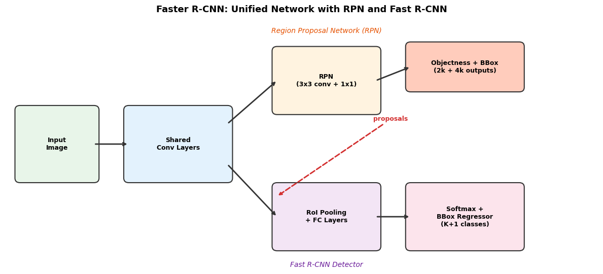
    (0.3, 2.0, 1.5, 1.5, 'Input\nImage', '#E8F5E9'),
    (2.5, 2.0, 2.0, 1.5, 'Shared\nConv Layers', '#E3F2FD'),
]

# RPN branch (top)
boxes_rpn = [
    (5.5, 3.5, 2.0, 1.3, 'RPN\n(3x3 conv + 1x1)', '#FFF3E0'),
    (8.2, 4.0, 2.2, 0.9, 'Objectness + BBox\n(2k + 4k outputs)', '#FFCCBC'),
]

# Detection branch (bottom)
boxes_det = [
    (5.5, 0.5, 2.0, 1.3, 'RoI Pooling\n+ FC Layers', '#F3E5F5'),
    (8.2, 0.5, 2.2, 1.3, 'Softmax +\nBBox Regressor\n(K+1 classes)', '#FCE4EC'),
]

for x, y, w, h, text, color in boxes_main + boxes_rpn + boxes_det:
    rect = mpatches.FancyBboxPatch(
        (x, y), w, h, boxstyle="round,pad=0.1",
        facecolor=color, edgecolor='#333333', linewidth=1.5
    )
    ax.add_patch(rect)
    ax.text(x + w/2, y + h/2, text,
            ha='center', va='center', fontsize=9, fontweight='bold')

# Arrows
arrow_style = dict(arrowstyle='->', color='#333333', lw=2)
ax.annotate('', xy=(2.5, 2.75), xytext=(1.8, 2.75), arrowprops=arrow_style)

# Shared conv to RPN
ax.annotate('', xy=(5.5, 4.15), xytext=(4.5, 3.2),
            arrowprops=arrow_style)
# Shared conv to detection
ax.annotate('', xy=(5.5, 1.15), xytext=(4.5, 2.3),
            arrowprops=arrow_style)

# RPN outputs
ax.annotate('', xy=(8.2, 4.45), xytext=(7.5, 4.15), arrowprops=arrow_style)
# Detection outputs
ax.annotate('', xy=(8.2, 1.15), xytext=(7.5, 1.15), arrowprops=arrow_style)

# RPN proposals feed into detection
ax.annotate('proposals', xy=(5.5, 1.6), xytext=(7.8, 3.3),
            arrowprops=dict(arrowstyle='->', color='#D32F2F', lw=2, linestyle='dashed'),
            fontsize=9, color='#D32F2F', fontweight='bold',
            ha='center', va='center')

# Labels
ax.text(6.5, 5.2, 'Region Proposal Network (RPN)',
        fontsize=10, fontstyle='italic', ha='center', color='#E65100')
ax.text(6.5, 0.05, 'Fast R-CNN Detector',
        fontsize=10, fontstyle='italic', ha='center', color='#6A1B9A')

ax.set_title('Faster R-CNN: Unified Network with RPN and Fast R-CNN',
             fontsize=13, fontweight='bold', pad=10)
plt.tight_layout()
plt.show()

3.3 Anchor Boxes

At each feature map location, the RPN defines \(k = 9\) anchor boxes using 3 scales and 3 aspect ratios:

• Scales: \(128^2\), \(256^2\), \(512^2\) pixels
• Aspect ratios: \(1:1\), \(1:2\), \(2:1\)

This design has several advantages:

• Pyramid of regression references on a single-scale feature map, avoiding the need for image pyramids or filter pyramids.
• Translation invariant by design: if an object translates in the image, the proposal translates with it and the same function predicts it. This contrasts with MultiBox, which uses k-means to generate 800 non-translation-invariant anchors.
• Far fewer parameters: The RPN output layer has approximately \(2.8 \times 10^4\) parameters (\(512 \times (4+2) \times 9\) for VGG-16), compared to \(6.1 \times 10^6\) for MultiBox — two orders of magnitude fewer.

import numpy as np

fig, axes = plt.subplots(1, 3, figsize=(12, 4))

scales = [128, 256, 512]
aspect_ratios = [(1, 1), (1, 2), (2, 1)]
ratio_labels = ['1:1', '1:2', '2:1']
colors = ['#1976D2', '#388E3C', '#D32F2F']

for idx, (scale, ax) in enumerate(zip(scales, axes)):
    ax.set_xlim(-350, 350)
    ax.set_ylim(-350, 350)
    ax.set_aspect('equal')
    ax.axhline(0, color='gray', lw=0.5, ls='--')
    ax.axvline(0, color='gray', lw=0.5, ls='--')
    ax.set_title(f'Scale: {scale}x{scale}', fontsize=11, fontweight='bold')

    for (ar_w, ar_h), color, label in zip(aspect_ratios, colors, ratio_labels):
        area = scale * scale
        w = np.sqrt(area * ar_w / ar_h)
        h = area / w
        rect = plt.Rectangle(
            (-w/2, -h/2), w, h,
            fill=False, edgecolor=color, linewidth=2, label=f'{label}'
        )
        ax.add_patch(rect)

    ax.plot(0, 0, 'ko', markersize=5)
    if idx == 2:
        ax.legend(loc='upper right', fontsize=9)
    ax.set_xlabel('pixels')

fig.suptitle('Anchor Boxes: 3 Scales x 3 Aspect Ratios = 9 Anchors per Location',
             fontsize=12, fontweight='bold', y=1.02)
plt.tight_layout()
plt.show()

3.4 RPN Training

The RPN uses a multi-task loss with the same structure as Fast R-CNN:

\[L(\{p_i\}, \{t_i\}) = \frac{1}{N_{\text{cls}}} \sum_i L_{\text{cls}}(p_i, p_i^*) + \lambda \frac{1}{N_{\text{reg}}} \sum_i p_i^* L_{\text{reg}}(t_i, t_i^*)\]

where \(p_i\) is the predicted objectness probability, \(p_i^*\) is the ground-truth label, \(t_i\) is the predicted box offsets, and \(t_i^*\) is the target offsets.

Anchor labeling:

• Positive: IoU \(> 0.7\) with any ground-truth box (or the highest IoU anchor for each ground-truth box)
• Negative: IoU \(< 0.3\) with all ground-truth boxes
• Anchors between 0.3 and 0.7 are ignored during training

Each mini-batch samples 256 anchors from a single image, with up to a 1:1 positive-to-negative ratio.

3.5 Sharing Features Between RPN and Fast R-CNN

Since both the RPN and the Fast R-CNN detector modify convolutional layers during training, a special procedure is needed to share features. The paper proposes a 4-step alternating training algorithm:

1. Train RPN from an ImageNet-pre-trained model, fine-tuning end-to-end for the region proposal task.
2. Train Fast R-CNN using RPN proposals, initialized separately from an ImageNet-pre-trained model. At this point the two networks do not share convolutional layers.
3. Re-initialize RPN with the detector network weights, and fine-tune only the RPN-unique layers (shared conv layers are now fixed).
4. Fine-tune Fast R-CNN unique layers, keeping the shared conv layers fixed.

The result is a unified network where convolutional features are shared between proposal generation and detection. Approximate joint training is also possible and is simpler, 25–50% faster, with similar accuracy.

3.6 Results

Near cost-free proposals. The RPN adds only ~10ms per image on top of the shared convolutional computation.

Speed comparison (VGG-16):

fig, (ax1, ax2) = plt.subplots(1, 2, figsize=(12, 4))

# Timing comparison
systems = ['R-CNN\n(VGG16)', 'SS + Fast R-CNN\n(VGG16)', 'Faster R-CNN\n(VGG16)']
times = [47000, 1830, 198]  # ms per image
bar_colors = ['#EF5350', '#FFA726', '#66BB6A']

bars = ax1.bar(systems, times, color=bar_colors, edgecolor='#333333', linewidth=1.2)
ax1.set_ylabel('Time per image (ms)', fontsize=11)
ax1.set_title('Test-Time Speed', fontsize=12, fontweight='bold')
ax1.set_yscale('log')
for bar, t in zip(bars, times):
    ax1.text(bar.get_x() + bar.get_width()/2., bar.get_height() * 1.1,
             f'{t}ms', ha='center', va='bottom', fontweight='bold', fontsize=10)

# mAP comparison
methods = ['R-CNN', 'Fast\nR-CNN', 'Faster\nR-CNN']
mAP_vals = [66.0, 66.9, 73.2]
bar_colors2 = ['#EF5350', '#FFA726', '#66BB6A']

bars2 = ax2.bar(methods, mAP_vals, color=bar_colors2, edgecolor='#333333', linewidth=1.2)
ax2.set_ylabel('mAP (%)', fontsize=11)
ax2.set_title('VOC 2007 mAP', fontsize=12, fontweight='bold')
ax2.set_ylim(60, 78)
for bar, v in zip(bars2, mAP_vals):
    ax2.text(bar.get_x() + bar.get_width()/2., bar.get_height() + 0.3,
             f'{v}%', ha='center', va='bottom', fontweight='bold', fontsize=11)

plt.suptitle('R-CNN Family: Speed and Accuracy Progression', fontsize=13, fontweight='bold', y=1.02)
plt.tight_layout()
plt.show()

Key results:

• Total system time: 198ms per image (5 fps) with VGG-16, vs. 1830ms for Selective Search + Fast R-CNN (0.5 fps) — a 10x speedup.
• Better accuracy: 73.2% mAP on VOC 2007 (using 07+12 training data) vs. 70.0% for Selective Search + Fast R-CNN.
• Only 300 proposals needed (vs. 2000 for Selective Search), with better recall characteristics.
• Two-stage detection (RPN + classifier) outperforms one-stage detection by approximately 5 mAP points.

3.7 Broader Impact

Faster R-CNN became the foundation for 1st-place entries in the ILSVRC and COCO 2015 competitions across detection, localization, and segmentation tracks. It benefits directly from deeper networks: replacing VGG-16 with ResNet-101 boosts mAP from 41.5% to 48.4% on the COCO dataset. The system was also adopted in commercial applications such as Pinterest’s visual search.

---

4. Summary: Evolution Across the Three Papers

import pandas as pd

data = {
    'Aspect': [
        'Region Proposals',
        'Feature Extraction',
        'Classifier',
        'BBox Regressor',
        'Training',
        'Test Speed (VGG16)',
        'VOC 2007 mAP',
        'Key Bottleneck',
    ],
    'R-CNN (2013)': [
        'Selective Search (external, CPU)',
        'Per-proposal CNN forward pass',
        'Linear SVMs (post-hoc)',
        'Separate stage',
        'Multi-stage pipeline',
        '~47s/image',
        '66.0%',
        'Per-proposal CNN passes',
    ],
    'Fast R-CNN (2015)': [
        'Selective Search (external, CPU)',
        'Single forward pass, RoI pooling',
        'Softmax (end-to-end)',
        'Joint multi-task loss',
        'Single-stage, multi-task',
        '~0.3s/image (excl. proposals)',
        '66.9%',
        'External region proposals',
    ],
    'Faster R-CNN (2015)': [
        'RPN (learned, GPU, shared features)',
        'Single forward pass, shared with RPN',
        'Softmax (end-to-end)',
        'Joint multi-task loss',
        '4-step alternating (or joint)',
        '~0.2s/image (incl. proposals)',
        '73.2% (07+12 data)',
        '-- (near real-time)',
    ],
}

df = pd.DataFrame(data)
df.style.set_properties(**{'text-align': 'left'}).set_table_styles([
    {'selector': 'th', 'props': [('text-align', 'left'), ('font-weight', 'bold')]}
])

	Aspect	R-CNN (2013)	Fast R-CNN (2015)	Faster R-CNN (2015)
0	Region Proposals	Selective Search (external, CPU)	Selective Search (external, CPU)	RPN (learned, GPU, shared features)
1	Feature Extraction	Per-proposal CNN forward pass	Single forward pass, RoI pooling	Single forward pass, shared with RPN
2	Classifier	Linear SVMs (post-hoc)	Softmax (end-to-end)	Softmax (end-to-end)
3	BBox Regressor	Separate stage	Joint multi-task loss	Joint multi-task loss
4	Training	Multi-stage pipeline	Single-stage, multi-task	4-step alternating (or joint)
5	Test Speed (VGG16)	~47s/image	~0.3s/image (excl. proposals)	~0.2s/image (incl. proposals)
6	VOC 2007 mAP	66.0%	66.9%	73.2% (07+12 data)
7	Key Bottleneck	Per-proposal CNN passes	External region proposals	-- (near real-time)

Key Recurring Themes

Looking across all three papers, four interconnected themes drive the improvements:

1. Feature sharing is the central driver of speed improvements. R-CNN computes features independently per proposal. Fast R-CNN shares convolutional computation across proposals. Faster R-CNN shares features between proposal generation and detection.

2. Multi-task learning (classification + regression) consistently outperforms stage-wise training. Joint optimization through a shared representation produces better features than training tasks in isolation.

3. Transfer learning from ImageNet pre-training remains essential throughout. Every model in the family is initialized from an ImageNet-pre-trained network and fine-tuned for detection.

4. End-to-end training produces better representations than pipelined approaches. The progression from separate SVMs and regressors (R-CNN) to a single unified network (Faster R-CNN) consistently improves both accuracy and efficiency.

The arc from R-CNN to Faster R-CNN demonstrates a broader principle: progressively replacing hand-designed components with learned alternatives — from external region proposals to learned RPNs, from separate SVMs to end-to-end softmax classifiers — unifies the system and lets the network learn jointly what was previously engineered in isolation.