YOLO: You Only Look Once — From v1 to v2

object-detection
deep-learning
computer-vision
real-time
A technical walkthrough of the YOLO family of real-time object detectors, tracing the evolution from YOLOv1 (2015) to YOLOv2/YOLO9000 (2016), covering unified detection as regression, the multi-part loss function, Darknet-19, anchor boxes with dimension clusters, and joint detection-classification training via WordTree.
Author

Ken Pu

Published

January 29, 2026

Introduction

By 2015, the dominant approach to object detection followed a multi-stage pipeline: generate region proposals, extract features per region, classify each proposal, and refine bounding boxes in a post-processing step. Systems like R-CNN took approximately 40 seconds per image. Even the faster variants — Fast R-CNN and Faster R-CNN — operated at only 0.5–7 FPS, well below real-time requirements.

The YOLO (You Only Look Once) family of detectors introduced a fundamentally different paradigm: object detection as a single regression problem. Instead of a complex pipeline of proposal generation, feature extraction, classification, and post-processing, YOLO runs a single neural network on the full image to directly predict bounding box coordinates and class probabilities.

This article covers two papers that define the YOLO approach:

  1. YOLOv1 (Redmon et al., 2015): Introduced the unified detection framework — a single convolutional network that reasons globally about the full image, achieving 45 FPS with 63.4% mAP on PASCAL VOC 2007.
  2. YOLOv2 / YOLO9000 (Redmon & Farhadi, 2016): Systematically addressed v1’s weaknesses through batch normalization, anchor boxes with learned dimension priors, multi-scale training, and a new backbone (Darknet-19), reaching 78.6% mAP at 40 FPS. The paper also introduced YOLO9000, which jointly trains on detection and classification data to detect over 9000 object categories in real-time.
Method mAP (VOC 2007) FPS Approach
R-CNN 66.0% 0.02 Multi-stage pipeline
Fast R-CNN 70.0% 0.5 Shared features, RoI pooling
Faster R-CNN (VGG-16) 73.2% 7 Learned proposals (RPN)
YOLOv1 63.4% 45 Single regression network
YOLOv2 (544) 78.6% 40 Improved single-shot

The key insight across both papers is that speed and accuracy are not inherently opposed — with the right architectural choices, a single-shot detector can match or exceed multi-stage detectors while running at real-time speeds.

1. YOLOv1: Unified Detection

1.1 Detection as Regression

YOLOv1’s fundamental contribution is reframing object detection as a single regression problem. The entire detection pipeline — feature extraction, bounding box prediction, class probability estimation, and non-maximum suppression — is collapsed into a single neural network evaluation.

The system works as follows:

  1. Divide the input image into an \(S \times S\) grid (with \(S = 7\) for PASCAL VOC).
  2. Each grid cell is responsible for detecting objects whose center falls within that cell.
  3. Each grid cell predicts:
    • \(B\) bounding boxes (\(B = 2\)), each with 5 values: \((x, y, w, h, \text{confidence})\)
    • \(C\) conditional class probabilities: \(\Pr(\text{Class}_i \mid \text{Object})\) (with \(C = 20\) for VOC)

The output is a single tensor of shape:

\[S \times S \times (B \cdot 5 + C) = 7 \times 7 \times 30\]

1.2 Confidence Score

Each bounding box has an associated confidence score defined as:

\[\text{Confidence} = \Pr(\text{Object}) \times \text{IOU}_{\text{pred}}^{\text{truth}}\]

If no object exists in a cell, the confidence should be zero. Otherwise, the confidence equals the IoU between the predicted box and the ground truth.

At test time, the class-specific confidence for each box is computed by combining the conditional class probability with the box confidence:

\[\Pr(\text{Class}_i \mid \text{Object}) \times \Pr(\text{Object}) \times \text{IOU}_{\text{pred}}^{\text{truth}} = \Pr(\text{Class}_i) \times \text{IOU}_{\text{pred}}^{\text{truth}} \tag{1}\]

This encodes both the probability that a particular class appears in the box and how well the predicted box fits the object.

Show code
import matplotlib.pyplot as plt
import matplotlib.patches as mpatches
import matplotlib.patches as patches
import numpy as np

fig, ax = plt.subplots(figsize=(10, 10))
ax.set_xlim(0, 10)
ax.set_ylim(0, 10)
ax.set_aspect('equal')
ax.set_title('YOLOv1: Grid-Based Detection (S=7)', fontsize=14, fontweight='bold', pad=15)

# Draw 7x7 grid
S = 7
cell_size = 10.0 / S
for i in range(S + 1):
    ax.axhline(i * cell_size, color='#BDBDBD', linewidth=0.8)
    ax.axvline(i * cell_size, color='#BDBDBD', linewidth=0.8)

# Draw a "ground truth" object (e.g., a dog)
gt_x, gt_y, gt_w, gt_h = 3.2, 2.5, 3.5, 4.0
gt_rect = patches.Rectangle((gt_x, gt_y), gt_w, gt_h, linewidth=2.5,
                             edgecolor='#4CAF50', facecolor='#4CAF50', alpha=0.12)
ax.add_patch(gt_rect)
ax.text(gt_x + gt_w / 2, gt_y + gt_h + 0.2, 'Ground Truth', ha='center',
        fontsize=10, color='#4CAF50', fontweight='bold')

# Highlight the responsible grid cell (center of object)
center_x = gt_x + gt_w / 2  # 4.95
center_y = gt_y + gt_h / 2  # 4.5
cell_col = int(center_x / cell_size)  # column 3
cell_row = int(center_y / cell_size)  # row 3
responsible_rect = patches.Rectangle(
    (cell_col * cell_size, cell_row * cell_size), cell_size, cell_size,
    linewidth=2.5, edgecolor='#F44336', facecolor='#F44336', alpha=0.25
)
ax.add_patch(responsible_rect)
ax.plot(center_x, center_y, 'r*', markersize=15, zorder=5)
ax.text(cell_col * cell_size + cell_size / 2, cell_row * cell_size + cell_size / 2 - 0.35,
        'Responsible\ncell', ha='center', va='center', fontsize=8, color='#D32F2F', fontweight='bold')

# Draw two predicted bounding boxes from the responsible cell
pred1 = patches.Rectangle((3.0, 2.8), 3.8, 3.6, linewidth=2, linestyle='--',
                           edgecolor='#1976D2', facecolor='none')
pred2 = patches.Rectangle((3.5, 2.2), 3.0, 4.5, linewidth=2, linestyle='--',
                           edgecolor='#FF9800', facecolor='none')
ax.add_patch(pred1)
ax.add_patch(pred2)

# Legend
legend_elements = [
    patches.Patch(facecolor='#4CAF50', alpha=0.3, edgecolor='#4CAF50', label='Ground truth box'),
    patches.Patch(facecolor='#F44336', alpha=0.3, edgecolor='#F44336', label='Responsible grid cell'),
    plt.Line2D([0], [0], color='#1976D2', linewidth=2, linestyle='--', label='Predicted box 1 (B=1)'),
    plt.Line2D([0], [0], color='#FF9800', linewidth=2, linestyle='--', label='Predicted box 2 (B=2)'),
    plt.Line2D([0], [0], marker='*', color='r', markersize=12, linestyle='None', label='Object center'),
]
ax.legend(handles=legend_elements, loc='upper right', fontsize=9, framealpha=0.9)

# Output tensor annotation
ax.text(5, 0.3, 'Output tensor: $7 \\times 7 \\times (2 \\cdot 5 + 20) = 7 \\times 7 \\times 30$',
        ha='center', fontsize=11, style='italic',
        bbox=dict(boxstyle='round,pad=0.4', facecolor='#FFF9C4', edgecolor='#F9A825'))

ax.set_xlabel('Image width', fontsize=11)
ax.set_ylabel('Image height', fontsize=11)
ax.invert_yaxis()
plt.tight_layout()
plt.show()

2. YOLOv1 Network Architecture

The YOLOv1 network architecture is inspired by GoogLeNet but uses a simpler design: instead of inception modules, it employs alternating \(1 \times 1\) reduction layers followed by \(3 \times 3\) convolutional layers. The full network has:

  • 24 convolutional layers for feature extraction
  • 2 fully connected layers for prediction

The first 20 convolutional layers are pre-trained on ImageNet at \(224 \times 224\) resolution (achieving 88% top-5 accuracy), then the full network is fine-tuned for detection at \(448 \times 448\) resolution. Four additional convolutional layers and two fully connected layers are added with randomly initialized weights.

A lightweight variant, Fast YOLO, uses only 9 convolutional layers with fewer filters, achieving 155 FPS with 52.7% mAP.

Show code
import matplotlib.pyplot as plt
import matplotlib.patches as patches

fig, ax = plt.subplots(figsize=(16, 4.5))
ax.set_xlim(0, 16)
ax.set_ylim(0, 4.5)
ax.axis('off')
ax.set_title('YOLOv1 Architecture: 24 Conv + 2 FC Layers', fontsize=14, fontweight='bold', pad=15)

# Define architecture blocks: (x, y, w, h, label, color, sublabel)
blocks = [
    (0.2, 0.8, 1.2, 2.8, 'Input\n448x448x3', '#FFE0B2', ''),
    (1.7, 1.0, 1.3, 2.4, 'Conv 7x7\n64, s=2\n+ Pool', '#BBDEFB', '224x224'),
    (3.3, 1.2, 1.2, 2.0, 'Conv 3x3\n192\n+ Pool', '#BBDEFB', '112x112'),
    (4.8, 1.3, 1.5, 1.8, '4x [1x1, 3x3]\n128-256\n512 + Pool', '#C8E6C9', '56x56'),
    (6.6, 1.4, 1.5, 1.6, '2x [1x1, 3x3]\n256-512\n1024 + Pool', '#C8E6C9', '28x28'),
    (8.4, 1.5, 1.5, 1.4, '2x [1x1, 3x3]\n512-1024\n+ 3x3, s=2', '#E1BEE7', '14x14'),
    (10.2, 1.6, 1.3, 1.2, '2x Conv\n3x3x1024', '#E1BEE7', '7x7'),
    (11.8, 1.7, 1.1, 1.0, 'FC\n4096', '#FFCDD2', ''),
    (13.2, 1.8, 1.1, 0.9, 'FC\n7x7x30', '#FFCDD2', ''),
    (14.6, 1.85, 1.1, 0.8, 'Output\n7x7x30', '#FFF9C4', ''),
]

for x, y, w, h, label, color, sublabel in blocks:
    rect = patches.FancyBboxPatch((x, y), w, h, boxstyle='round,pad=0.08',
                                  facecolor=color, edgecolor='#555555', linewidth=1.2)
    ax.add_patch(rect)
    ax.text(x + w/2, y + h/2, label, ha='center', va='center', fontsize=7, fontweight='bold')
    if sublabel:
        ax.text(x + w/2, y - 0.15, sublabel, ha='center', fontsize=6, color='#666666', style='italic')

# Arrows
arrow_xs = [(1.4, 1.7), (3.0, 3.3), (4.5, 4.8), (6.3, 6.6), (8.1, 8.4),
            (9.9, 10.2), (11.5, 11.8), (12.9, 13.2), (14.3, 14.6)]
for x1, x2 in arrow_xs:
    ax.annotate('', xy=(x2, 2.2), xytext=(x1, 2.2),
                arrowprops=dict(arrowstyle='->', color='#555555', lw=1.5))

# Pre-training bracket
ax.annotate('', xy=(1.7, 3.9), xytext=(8.1, 3.9),
            arrowprops=dict(arrowstyle='<->', color='#1565C0', lw=1.5))
ax.text(4.9, 4.15, 'Pre-trained on ImageNet (first 20 conv layers, 224x224)',
        ha='center', fontsize=8, color='#1565C0', fontweight='bold')

# Detection bracket
ax.annotate('', xy=(8.4, 0.4), xytext=(14.6, 0.4),
            arrowprops=dict(arrowstyle='<->', color='#C62828', lw=1.5))
ax.text(11.5, 0.15, 'Added for detection (448x448)',
        ha='center', fontsize=8, color='#C62828', fontweight='bold')

plt.tight_layout()
plt.show()

3. YOLOv1 Training

3.1 Multi-Part Loss Function

YOLOv1 uses a sum-squared error loss composed of five terms. The choice of sum-squared error is motivated by ease of optimization, though it requires careful weighting to balance localization, confidence, and classification objectives.

The full loss function (Equation 3 from the paper) is:

\[\mathcal{L} = \underbrace{\lambda_{\text{coord}} \sum_{i=0}^{S^2} \sum_{j=0}^{B} \mathbb{1}_{ij}^{\text{obj}} \left[ (x_i - \hat{x}_i)^2 + (y_i - \hat{y}_i)^2 \right]}_{\text{Center coordinate loss}}\]

\[+ \underbrace{\lambda_{\text{coord}} \sum_{i=0}^{S^2} \sum_{j=0}^{B} \mathbb{1}_{ij}^{\text{obj}} \left[ \left(\sqrt{w_i} - \sqrt{\hat{w}_i}\right)^2 + \left(\sqrt{h_i} - \sqrt{\hat{h}_i}\right)^2 \right]}_{\text{Width/height loss (square root)}}\]

\[+ \underbrace{\sum_{i=0}^{S^2} \sum_{j=0}^{B} \mathbb{1}_{ij}^{\text{obj}} \left( C_i - \hat{C}_i \right)^2}_{\text{Confidence loss (object)}}\]

\[+ \underbrace{\lambda_{\text{noobj}} \sum_{i=0}^{S^2} \sum_{j=0}^{B} \mathbb{1}_{ij}^{\text{noobj}} \left( C_i - \hat{C}_i \right)^2}_{\text{Confidence loss (no object)}}\]

\[+ \underbrace{\sum_{i=0}^{S^2} \mathbb{1}_i^{\text{obj}} \sum_{c \in \text{classes}} \left( p_i(c) - \hat{p}_i(c) \right)^2}_{\text{Classification loss}}\]

where:

  • \(\mathbb{1}_{ij}^{\text{obj}}\) indicates the \(j\)-th bounding box predictor in cell \(i\) is “responsible” for an object (has highest IOU with ground truth)
  • \(\lambda_{\text{coord}} = 5\) increases the weight of coordinate predictions
  • \(\lambda_{\text{noobj}} = 0.5\) decreases the weight of confidence loss for cells without objects
  • Square roots of \(w\) and \(h\) are predicted to reduce sensitivity to size: small deviations in large boxes matter less than in small boxes

3.2 Predictor Responsibility

At training time, only one bounding box predictor per grid cell is assigned responsibility for each ground truth object — the one with the highest current IoU with the ground truth. This leads to specialization: each predictor gets better at predicting certain sizes, aspect ratios, or classes.

3.3 Activation Function

All layers (except the final output layer, which uses a linear activation) use the leaky ReLU activation:

\[\phi(x) = \begin{cases} x & \text{if } x > 0 \\ 0.1x & \text{otherwise} \end{cases}\]

3.4 Training Schedule and Augmentation

  • Learning rate warm-up: Start at \(10^{-3}\), slowly raise to \(10^{-2}\) during the first epochs to prevent early divergence from unstable gradients.
  • Continue with \(10^{-2}\) for 75 epochs, then \(10^{-3}\) for 30 epochs, and \(10^{-4}\) for 30 epochs.
  • Dropout with rate 0.5 after the first fully connected layer.
  • Data augmentation: random scaling and translations (up to 20% of image size), random adjustments to exposure and saturation in HSV color space (up to factor 1.5).
  • Trained for ~135 epochs on VOC 2007+2012 training data.

4. YOLOv1 Results and Properties

4.1 Speed

YOLOv1 achieves true real-time performance:

  • YOLO: 45 FPS (22ms per image) on a Titan X GPU
  • Fast YOLO: 155 FPS (6.4ms per image) — the fastest general-purpose object detector at the time

4.2 Detection Results on VOC 2007

Show code
import pandas as pd

data = {
    'Method': [
        '100Hz DPM', '30Hz DPM', 'Fast YOLO', 'YOLO',
        'Fastest DPM', 'R-CNN Minus R', 'Fast R-CNN',
        'Faster R-CNN VGG-16', 'Faster R-CNN ZF', 'YOLO VGG-16'
    ],
    'Train Data': [
        '2007', '2007', '2007+2012', '2007+2012',
        '2007', '2007', '2007+2012',
        '2007+2012', '2007+2012', '2007+2012'
    ],
    'mAP': [16.0, 26.1, 52.7, 63.4, 30.4, 53.5, 70.0, 73.2, 62.1, 66.4],
    'FPS': [100, 30, 155, 45, 15, 6, 0.5, 7, 18, 21],
    'Real-Time': ['Yes', 'Yes', 'Yes', 'Yes', 'No', 'No', 'No', 'No', 'No', 'No']
}
df = pd.DataFrame(data)
df.style.set_properties(**{'text-align': 'center'}).set_table_styles([
    {'selector': 'th', 'props': [('text-align', 'center'), ('font-weight', 'bold')]}
]).set_caption('Table 1: Real-Time Systems on PASCAL VOC 2007')
Table 1: Table 1: Real-Time Systems on PASCAL VOC 2007
  Method Train Data mAP FPS Real-Time
0 100Hz DPM 2007 16.000000 100.000000 Yes
1 30Hz DPM 2007 26.100000 30.000000 Yes
2 Fast YOLO 2007+2012 52.700000 155.000000 Yes
3 YOLO 2007+2012 63.400000 45.000000 Yes
4 Fastest DPM 2007 30.400000 15.000000 No
5 R-CNN Minus R 2007 53.500000 6.000000 No
6 Fast R-CNN 2007+2012 70.000000 0.500000 No
7 Faster R-CNN VGG-16 2007+2012 73.200000 7.000000 No
8 Faster R-CNN ZF 2007+2012 62.100000 18.000000 No
9 YOLO VGG-16 2007+2012 66.400000 21.000000 No

4.3 Error Analysis: YOLO vs Fast R-CNN

A detailed error analysis using the Hoiem et al. methodology reveals the complementary error profiles of YOLO and Fast R-CNN. The categories of errors are:

  • Correct: correct class and IoU > 0.5
  • Localization: correct class, 0.1 < IoU < 0.5
  • Similar: similar class, IoU > 0.1
  • Other: wrong class, IoU > 0.1
  • Background: IoU < 0.1 for any object
Show code
import matplotlib.pyplot as plt
import numpy as np

fig, axes = plt.subplots(1, 2, figsize=(12, 5))

# Error breakdown data from Figure 4 of YOLOv1 paper
categories = ['Correct', 'Localization', 'Similar', 'Other', 'Background']
fast_rcnn_vals = [71.6, 8.6, 4.3, 1.9, 13.6]
yolo_vals = [65.5, 19.0, 6.75, 4.0, 4.75]
colors = ['#4CAF50', '#FF9800', '#2196F3', '#9C27B0', '#F44336']

# Fast R-CNN
wedges1, texts1, autotexts1 = axes[0].pie(
    fast_rcnn_vals, labels=categories, colors=colors, autopct='%1.1f%%',
    startangle=90, textprops={'fontsize': 9}
)
axes[0].set_title('Fast R-CNN', fontsize=13, fontweight='bold')

# YOLO
wedges2, texts2, autotexts2 = axes[1].pie(
    yolo_vals, labels=categories, colors=colors, autopct='%1.1f%%',
    startangle=90, textprops={'fontsize': 9}
)
axes[1].set_title('YOLO', fontsize=13, fontweight='bold')

fig.suptitle('Error Analysis: Fast R-CNN vs YOLO (VOC 2007)',
             fontsize=14, fontweight='bold', y=1.02)
plt.tight_layout()
plt.show()

The error analysis reveals two key findings:

  1. YOLO’s dominant error is localization (19.0% vs 8.6% for Fast R-CNN). This is the primary weakness of the grid-based approach.
  2. Fast R-CNN’s dominant error is background false positives (13.6% vs 4.75% for YOLO). Because Fast R-CNN operates on local patches, it cannot reason about global context. YOLO sees the entire image, making it far less likely to mistake background for objects.

4.4 Complementarity with R-CNN

Because YOLO and Fast R-CNN make different kinds of errors, combining them produces a significant boost. For every bounding box predicted by Fast R-CNN, if YOLO also predicts a similar box, the prediction receives a confidence boost:

Model mAP Combined Gain
Fast R-CNN alone 71.8
+ YOLO 63.4 75.0 +3.2
+ Fast R-CNN (2007 data) 66.9 72.4 +0.6
+ Fast R-CNN (VGG-M) 59.2 72.4 +0.6

The 3.2% boost from YOLO is far larger than the boost from other Fast R-CNN variants, confirming that the improvement comes from the complementary error profiles, not just model ensembling.

4.5 Generalization to Artwork

YOLO generalizes better to new domains than R-CNN. On the Picasso Dataset and People-Art Dataset (person detection on artwork), YOLO substantially outperforms R-CNN:

Method VOC 2007 AP Picasso AP People-Art AP
YOLO 59.2 53.3 45
R-CNN 54.2 10.4 26
DPM 43.2 37.8 32

R-CNN depends on Selective Search, which is tuned for natural images and fails on artwork. YOLO models the size, shape, and layout of objects globally, which transfers across domains.

5. YOLOv1 Limitations

Despite its speed advantages, YOLOv1 has several important limitations:

  1. Spatial constraint: Each grid cell predicts only 2 boxes and can have only 1 class. This limits the number of nearby objects that can be detected — the model struggles with small objects in groups (e.g., flocks of birds).

  2. Localization errors are dominant: 19% of errors come from localization, more than all other error sources combined. The coarse grid and fully connected output layers limit spatial precision.

  3. Coarse features: Multiple downsampling layers from the \(448 \times 448\) input to the \(7 \times 7\) feature map discard fine-grained spatial information.

  4. Scale sensitivity: The loss function treats errors equally for small and large boxes. Although the square root partially addresses this, small objects remain difficult.

These specific limitations directly motivate the improvements in YOLOv2.


6. YOLOv2 — Better: Systematic Improvements

YOLOv2 addresses each of YOLOv1’s weaknesses through a series of incremental improvements. The paper carefully traces the mAP impact of each change, building from 63.4% to 78.6%.

6.1 Path from YOLO to YOLOv2

Show code
import pandas as pd

improvements = {
    'Configuration': [
        'YOLO (baseline)',
        '+ Batch Normalization',
        '+ High-Res Classifier',
        '+ Convolutional (FC removed)',
        '+ Anchor Boxes',
        '+ New Network (Darknet-19)',
        '+ Dimension Priors',
        '+ Location Prediction',
        '+ Passthrough',
        '+ Multi-Scale',
        '+ Hi-Res Detector (544)',
    ],
    'VOC 2007 mAP': [63.4, 65.8, 69.5, 69.2, 69.6, 74.4, 75.4, 76.8, 76.8, 76.8, 78.6],
}
df_improvements = pd.DataFrame(improvements)
df_improvements.style.set_properties(**{'text-align': 'left'}).set_table_styles([
    {'selector': 'th', 'props': [('text-align', 'left'), ('font-weight', 'bold')]}
]).set_caption('Table 2: The path from YOLO to YOLOv2 (cumulative mAP on VOC 2007)')
Table 2: Table 2: The path from YOLO to YOLOv2 (cumulative mAP on VOC 2007)
  Configuration VOC 2007 mAP
0 YOLO (baseline) 63.400000
1 + Batch Normalization 65.800000
2 + High-Res Classifier 69.500000
3 + Convolutional (FC removed) 69.200000
4 + Anchor Boxes 69.600000
5 + New Network (Darknet-19) 74.400000
6 + Dimension Priors 75.400000
7 + Location Prediction 76.800000
8 + Passthrough 76.800000
9 + Multi-Scale 76.800000
10 + Hi-Res Detector (544) 78.600000
Show code
import matplotlib.pyplot as plt
import numpy as np

labels = [
    'YOLO\n(baseline)', '+BatchNorm', '+Hi-Res\nClassifier',
    '+Conv', '+Anchors', '+Darknet-19',
    '+Dim Priors', '+Loc Pred', '+Passthrough',
    '+Multi-Scale', '+Hi-Res\n(544)'
]
mAP_vals = [63.4, 65.8, 69.5, 69.2, 69.6, 74.4, 75.4, 76.8, 76.8, 76.8, 78.6]

fig, ax = plt.subplots(figsize=(14, 5))
colors = plt.cm.YlOrRd(np.linspace(0.2, 0.85, len(labels)))
bars = ax.bar(range(len(labels)), mAP_vals, color=colors, edgecolor='white', linewidth=1.5)

for i, (bar, val) in enumerate(zip(bars, mAP_vals)):
    ax.text(bar.get_x() + bar.get_width()/2, bar.get_height() + 0.3,
            f'{val}%', ha='center', va='bottom', fontweight='bold', fontsize=9)

ax.set_xticks(range(len(labels)))
ax.set_xticklabels(labels, fontsize=8, rotation=0)
ax.set_ylabel('mAP (%)', fontsize=12)
ax.set_title('The Path from YOLO to YOLOv2: Cumulative Improvements on VOC 2007',
             fontsize=13, fontweight='bold')
ax.set_ylim(58, 82)
ax.spines['top'].set_visible(False)
ax.spines['right'].set_visible(False)
ax.grid(axis='y', alpha=0.2)
plt.tight_layout()
plt.show()

6.2 Batch Normalization

Adding batch normalization to all convolutional layers yields:

  • +2% mAP improvement
  • Acts as a regularizer, allowing dropout to be removed without overfitting
  • Improves convergence during training

6.3 High Resolution Classifier

YOLOv1 pre-trained its classifier at \(224 \times 224\), then abruptly switched to \(448 \times 448\) for detection. YOLOv2 adds an intermediate step: fine-tune the classifier at \(448 \times 448\) for 10 epochs on ImageNet before switching to detection training. This gives the network time to adjust its filters to higher resolution input. Result: +4% mAP.

6.4 Anchor Boxes

YOLOv1 predicts bounding box coordinates directly through fully connected layers. YOLOv2 replaces this with anchor boxes (inspired by Faster R-CNN’s RPN):

  • Remove fully connected layers entirely
  • Shrink input from \(448 \times 448\) to \(416 \times 416\) to produce a \(13 \times 13\) feature map (odd dimensions ensure a single center cell for large objects)
  • Predict offsets from anchor priors instead of raw coordinates
  • Decouple class prediction from spatial location: predict class + objectness per anchor box

Result: mAP slightly decreased (69.5 to 69.2), but recall increased from 81% to 88%, providing more room for improvement.

6.5 Dimension Clusters

Rather than hand-picking anchor box dimensions (as in Faster R-CNN), YOLOv2 uses \(k\)-means clustering on the training set bounding boxes with a custom distance metric:

\[d(\text{box}, \text{centroid}) = 1 - \text{IOU}(\text{box}, \text{centroid})\]

Using standard Euclidean distance would bias toward larger boxes. The IOU-based distance is size-invariant and directly optimizes for what matters: overlap quality.

With \(k = 5\) priors, the cluster centroids achieve 61.0 Avg IOU, comparable to 60.9 for 9 hand-picked anchors from Faster R-CNN. Using \(k = 9\) clusters reaches 67.2 Avg IOU.

6.6 Direct Location Prediction

Faster R-CNN’s unconstrained offset predictions (\(x = t_x \cdot w_a - x_a\)) allow any anchor box to shift to any point in the image, causing model instability during early training.

YOLOv2 constrains the location prediction using sigmoid activation to bound the center coordinates within the grid cell:

Show code
import matplotlib.pyplot as plt
import matplotlib.patches as patches
import numpy as np

fig, ax = plt.subplots(figsize=(8, 8))
ax.set_xlim(-0.5, 4.5)
ax.set_ylim(-0.5, 4.5)
ax.set_aspect('equal')
ax.invert_yaxis()

# Draw grid
for i in range(5):
    ax.axhline(i, color='#BDBDBD', linewidth=1, linestyle='--')
    ax.axvline(i, color='#BDBDBD', linewidth=1, linestyle='--')

# Highlight the target cell (cx=1, cy=1)
cx, cy = 1, 1
cell_rect = patches.Rectangle((cx, cy), 1, 1, linewidth=2,
                               edgecolor='#1565C0', facecolor='#E3F2FD', alpha=0.5)
ax.add_patch(cell_rect)
ax.text(cx, cy - 0.1, f'($c_x={cx}$, $c_y={cy}$)', fontsize=10, color='#1565C0')

# Prior box (dashed)
pw, ph = 1.8, 2.5
sigma_tx, sigma_ty = 0.6, 0.4  # sigmoid outputs
bx = sigma_tx + cx
by = sigma_ty + cy
tw, th = 0.3, 0.2  # network predictions for width/height
bw = pw * np.exp(tw)
bh = ph * np.exp(th)

# Draw prior box centered at cell corner
prior_rect = patches.Rectangle(
    (cx + 0.5 - pw/2, cy + 0.5 - ph/2), pw, ph,
    linewidth=2, linestyle=':', edgecolor='#9E9E9E', facecolor='none'
)
ax.add_patch(prior_rect)
ax.text(cx + 0.5 + pw/2 + 0.1, cy + 0.5, f'Prior\n$p_w={pw}$, $p_h={ph}$',
        fontsize=9, color='#757575', va='center')

# Draw predicted box
pred_rect = patches.Rectangle(
    (bx - bw/2, by - bh/2), bw, bh,
    linewidth=2.5, edgecolor='#E53935', facecolor='#FFCDD2', alpha=0.3
)
ax.add_patch(pred_rect)
ax.plot(bx, by, 'ro', markersize=8, zorder=5)
ax.text(bx + 0.1, by + 0.15, f'($b_x$, $b_y$)', fontsize=10, color='#E53935', fontweight='bold')

# Annotations
ax.annotate(r'$\sigma(t_x)$', xy=(bx, cy + 0.5), xytext=(bx, cy + 0.95),
            fontsize=11, color='#E53935', ha='center',
            arrowprops=dict(arrowstyle='<->', color='#E53935', lw=1.5))
ax.annotate(r'$\sigma(t_y)$', xy=(cx + 0.5, by), xytext=(cx + 0.95, by),
            fontsize=11, color='#E53935', va='center',
            arrowprops=dict(arrowstyle='<->', color='#E53935', lw=1.5))

# Equations box
eq_text = (
    '$b_x = \\sigma(t_x) + c_x$\n'
    '$b_y = \\sigma(t_y) + c_y$\n'
    '$b_w = p_w e^{t_w}$\n'
    '$b_h = p_h e^{t_h}$'
)
ax.text(3.0, 0.2, eq_text, fontsize=11, va='top',
        bbox=dict(boxstyle='round,pad=0.4', facecolor='#FFF9C4', edgecolor='#F9A825', alpha=0.9))

ax.set_title('YOLOv2: Bounding Box Prediction with Dimension Priors',
             fontsize=13, fontweight='bold', pad=15)
ax.set_xlabel('Grid columns', fontsize=11)
ax.set_ylabel('Grid rows', fontsize=11)
plt.tight_layout()
plt.show()

The prediction equations are:

\[b_x = \sigma(t_x) + c_x \qquad b_y = \sigma(t_y) + c_y\] \[b_w = p_w e^{t_w} \qquad b_h = p_h e^{t_h}\] \[\Pr(\text{object}) \times \text{IOU}(b, \text{object}) = \sigma(t_o)\]

where \((c_x, c_y)\) is the top-left offset of the grid cell and \((p_w, p_h)\) is the prior box dimension from clustering. The sigmoid constrains the center to fall within the grid cell, stabilizing training. Combined with dimension clusters: +5% mAP over the anchor box baseline.

6.7 Fine-Grained Features (Passthrough Layer)

The \(13 \times 13\) feature map is sufficient for large objects but may miss small objects. YOLOv2 adds a passthrough layer that brings features from an earlier \(26 \times 26\) layer:

  • Adjacent spatial features are stacked into channels: \(26 \times 26 \times 512 \rightarrow 13 \times 13 \times 2048\)
  • This is concatenated with the \(13 \times 13\) feature map
  • Similar concept to skip connections in ResNet
  • Result: +1% mAP, particularly for smaller objects

6.8 Multi-Scale Training

Since YOLOv2 is fully convolutional (no FC layers), it can accept images of any size. During training, every 10 batches the network randomly switches to a new input resolution drawn from multiples of 32: \(\{320, 352, 384, \ldots, 608\}\).

This forces the network to learn scale-invariant predictions and offers a smooth speed/accuracy tradeoff at test time:

Input Size mAP (VOC 2007) FPS
288 x 288 69.0 91
352 x 352 73.7 81
416 x 416 76.8 67
480 x 480 77.8 59
544 x 544 78.6 40

7. YOLOv2 — Faster: Darknet-19

7.1 Backbone Comparison

Most detection frameworks at the time used VGG-16 as their backbone, which requires 30.69 billion floating point operations per forward pass. YOLOv2 introduces Darknet-19, a new backbone that is both faster and more accurate:

Backbone Billion FLOPs Top-5 Accuracy (ImageNet)
VGG-16 30.69 90.0%
YOLO (GoogLeNet-inspired) 8.52 88.0%
Darknet-19 5.58 91.2%

Darknet-19 achieves higher accuracy with 5.5x fewer operations than VGG-16.

7.2 Darknet-19 Architecture

Show code
import pandas as pd

darknet19 = {
    'Layer': [
        'Conv 1', 'Maxpool',
        'Conv 2', 'Maxpool',
        'Conv 3', 'Conv 4', 'Conv 5', 'Maxpool',
        'Conv 6', 'Conv 7', 'Conv 8', 'Maxpool',
        'Conv 9', 'Conv 10', 'Conv 11', 'Conv 12', 'Conv 13', 'Maxpool',
        'Conv 14', 'Conv 15', 'Conv 16', 'Conv 17', 'Conv 18',
        'Conv 19', 'Avgpool', 'Softmax'
    ],
    'Filters': [
        32, '--',
        64, '--',
        128, 64, 128, '--',
        256, 128, 256, '--',
        512, 256, 512, 256, 512, '--',
        1024, 512, 1024, 512, 1024,
        1000, '--', '--'
    ],
    'Size/Stride': [
        '3x3', '2x2/2',
        '3x3', '2x2/2',
        '3x3', '1x1', '3x3', '2x2/2',
        '3x3', '1x1', '3x3', '2x2/2',
        '3x3', '1x1', '3x3', '1x1', '3x3', '2x2/2',
        '3x3', '1x1', '3x3', '1x1', '3x3',
        '1x1', 'Global', '--'
    ],
    'Output': [
        '224x224', '112x112',
        '112x112', '56x56',
        '56x56', '56x56', '56x56', '28x28',
        '28x28', '28x28', '28x28', '14x14',
        '14x14', '14x14', '14x14', '14x14', '14x14', '7x7',
        '7x7', '7x7', '7x7', '7x7', '7x7',
        '7x7', '1000', '1000'
    ]
}
df_darknet = pd.DataFrame(darknet19)
df_darknet.style.set_properties(**{'text-align': 'center'}).set_table_styles([
    {'selector': 'th', 'props': [('text-align', 'center'), ('font-weight', 'bold')]}
]).set_caption('Table 6: Darknet-19 Architecture (19 conv + 5 maxpool layers)')
Table 3: Table 6: Darknet-19 Architecture (19 conv + 5 maxpool layers)
  Layer Filters Size/Stride Output
0 Conv 1 32 3x3 224x224
1 Maxpool -- 2x2/2 112x112
2 Conv 2 64 3x3 112x112
3 Maxpool -- 2x2/2 56x56
4 Conv 3 128 3x3 56x56
5 Conv 4 64 1x1 56x56
6 Conv 5 128 3x3 56x56
7 Maxpool -- 2x2/2 28x28
8 Conv 6 256 3x3 28x28
9 Conv 7 128 1x1 28x28
10 Conv 8 256 3x3 28x28
11 Maxpool -- 2x2/2 14x14
12 Conv 9 512 3x3 14x14
13 Conv 10 256 1x1 14x14
14 Conv 11 512 3x3 14x14
15 Conv 12 256 1x1 14x14
16 Conv 13 512 3x3 14x14
17 Maxpool -- 2x2/2 7x7
18 Conv 14 1024 3x3 7x7
19 Conv 15 512 1x1 7x7
20 Conv 16 1024 3x3 7x7
21 Conv 17 512 1x1 7x7
22 Conv 18 1024 3x3 7x7
23 Conv 19 1000 1x1 7x7
24 Avgpool -- Global 1000
25 Softmax -- -- 1000

7.3 Design Principles

Darknet-19 follows several established design principles:

  • 3x3 convolutions throughout (VGG-style), with channels doubled after each pooling step
  • 1x1 filters between 3x3 convolutions to compress feature representations (Network-in-Network style)
  • Batch normalization on every convolutional layer
  • Global average pooling for final predictions (no fully connected layers)

7.4 Training Pipeline

  1. Classification training: Train on ImageNet at \(224 \times 224\) for 160 epochs (SGD, lr=0.1, polynomial decay)
  2. High-resolution fine-tuning: Fine-tune at \(448 \times 448\) for 10 epochs (lr=\(10^{-3}\)) — achieves 76.5% top-1
  3. Detection adaptation: Remove last conv layer, add three \(3 \times 3 \times 1024\) conv layers + \(1 \times 1\) output layer
  4. Add passthrough from the \(3 \times 3 \times 512\) layer for fine-grained features

8. YOLOv2 Results

8.1 Detection Frameworks on VOC 2007

Show code
import pandas as pd

voc2007 = {
    'Method': [
        'Fast R-CNN', 'Faster R-CNN VGG-16', 'Faster R-CNN ResNet',
        'YOLO', 'SSD300', 'SSD512',
        'YOLOv2 288x288', 'YOLOv2 352x352', 'YOLOv2 416x416',
        'YOLOv2 480x480', 'YOLOv2 544x544'
    ],
    'Train Data': [
        '07+12', '07+12', '07+12',
        '07+12', '07+12', '07+12',
        '07+12', '07+12', '07+12', '07+12', '07+12'
    ],
    'mAP': [70.0, 73.2, 76.4, 63.4, 74.3, 76.8, 69.0, 73.7, 76.8, 77.8, 78.6],
    'FPS': [0.5, 7, 5, 45, 46, 19, 91, 81, 67, 59, 40]
}
df_voc = pd.DataFrame(voc2007)
df_voc.style.set_properties(**{'text-align': 'center'}).set_table_styles([
    {'selector': 'th', 'props': [('text-align', 'center'), ('font-weight', 'bold')]}
]).set_caption('Table 3: Detection Frameworks on PASCAL VOC 2007')
Table 4: Table 3: Detection Frameworks on PASCAL VOC 2007
  Method Train Data mAP FPS
0 Fast R-CNN 07+12 70.000000 0.500000
1 Faster R-CNN VGG-16 07+12 73.200000 7.000000
2 Faster R-CNN ResNet 07+12 76.400000 5.000000
3 YOLO 07+12 63.400000 45.000000
4 SSD300 07+12 74.300000 46.000000
5 SSD512 07+12 76.800000 19.000000
6 YOLOv2 288x288 07+12 69.000000 91.000000
7 YOLOv2 352x352 07+12 73.700000 81.000000
8 YOLOv2 416x416 07+12 76.800000 67.000000
9 YOLOv2 480x480 07+12 77.800000 59.000000
10 YOLOv2 544x544 07+12 78.600000 40.000000

8.2 Speed vs. Accuracy

Show code
import matplotlib.pyplot as plt
import numpy as np

fig, ax = plt.subplots(figsize=(10, 7))

# Data points
methods = [
    ('R-CNN', 0.05, 66.0, 's', '#EF5350'),
    ('Fast R-CNN', 0.5, 70.0, 's', '#EF5350'),
    ('Faster R-CNN\nVGG-16', 7, 73.2, 's', '#EF5350'),
    ('Faster R-CNN\nResNet', 5, 76.4, 's', '#EF5350'),
    ('YOLO', 45, 63.4, 'D', '#FFA726'),
    ('SSD300', 46, 74.3, '^', '#66BB6A'),
    ('SSD512', 19, 76.8, '^', '#66BB6A'),
]

# YOLOv2 multi-scale points
yolov2_fps = [91, 81, 67, 59, 40]
yolov2_mAP = [69.0, 73.7, 76.8, 77.8, 78.6]
yolov2_labels = ['288', '352', '416', '480', '544']

# Plot other methods
for name, fps, mAP, marker, color in methods:
    ax.scatter(fps, mAP, s=200, c=color, marker=marker, edgecolors='black',
               linewidth=1, zorder=5)
    offset_x = 2
    offset_y = 1.0
    if 'Faster' in name and 'ResNet' in name:
        offset_x = -8
        offset_y = -2.0
    elif 'Faster' in name:
        offset_x = -8
        offset_y = 1.0
    elif name == 'R-CNN':
        offset_x = 2
        offset_y = -2.0
    elif name == 'Fast R-CNN':
        offset_x = 2
        offset_y = -2.0
    elif name == 'SSD512':
        offset_x = -8
        offset_y = -2.0
    ax.annotate(f'{name}\n({mAP}%)', (fps, mAP),
                textcoords='offset points', xytext=(offset_x, offset_y),
                fontsize=8, fontweight='bold')

# Plot YOLOv2 line
ax.plot(yolov2_fps, yolov2_mAP, 'o-', color='#1565C0', markersize=10,
        markeredgecolor='black', markeredgewidth=1, linewidth=2, zorder=5,
        label='YOLOv2 (multi-scale)')
for fps, mAP, label in zip(yolov2_fps, yolov2_mAP, yolov2_labels):
    ax.annotate(f'{label}\n{mAP}%', (fps, mAP),
                textcoords='offset points', xytext=(3, 5),
                fontsize=8, color='#1565C0', fontweight='bold')

# Real-time threshold
ax.axvline(x=30, color='green', linestyle='--', alpha=0.4, linewidth=1.5)
ax.text(31, 62, 'Real-time\n(30 FPS)', fontsize=9, color='green', style='italic')

ax.set_xlabel('Frames Per Second (FPS)', fontsize=12)
ax.set_ylabel('mAP (%) on VOC 2007', fontsize=12)
ax.set_title('Speed vs. Accuracy on PASCAL VOC 2007 (Figure 4 from YOLOv2 paper)',
             fontsize=13, fontweight='bold')
ax.set_xlim(-2, 100)
ax.set_ylim(58, 82)
ax.spines['top'].set_visible(False)
ax.spines['right'].set_visible(False)
ax.grid(True, alpha=0.2)
ax.legend(loc='lower right', fontsize=10)
plt.tight_layout()
plt.show()

8.3 VOC 2012 Results

Show code
import pandas as pd

voc2012 = {
    'Method': [
        'Fast R-CNN', 'Faster R-CNN', 'YOLO',
        'SSD300', 'SSD512', 'ResNet', 'YOLOv2 544'
    ],
    'Train Data': ['07++12']*7,
    'mAP': [68.4, 70.4, 57.9, 72.4, 74.9, 73.8, 73.4],
}
df_voc12 = pd.DataFrame(voc2012)
df_voc12.style.set_properties(**{'text-align': 'center'}).set_table_styles([
    {'selector': 'th', 'props': [('text-align', 'center'), ('font-weight', 'bold')]}
]).set_caption('Table 4: PASCAL VOC 2012 Test Detection Results')
Table 5: Table 4: PASCAL VOC 2012 Test Detection Results
  Method Train Data mAP
0 Fast R-CNN 07++12 68.400000
1 Faster R-CNN 07++12 70.400000
2 YOLO 07++12 57.900000
3 SSD300 07++12 72.400000
4 SSD512 07++12 74.900000
5 ResNet 07++12 73.800000
6 YOLOv2 544 07++12 73.400000

8.4 COCO Results

Show code
import pandas as pd

coco = {
    'Method': [
        'Fast R-CNN', 'Faster R-CNN', 'SSD300', 'SSD512', 'YOLOv2'
    ],
    'mAP@[.5:.95]': [20.5, 24.2, 23.2, 26.8, 21.6],
    'mAP@0.5': [39.9, 45.3, 41.2, 46.5, 44.0],
    'mAP@0.75': [19.4, 23.5, 23.4, 27.8, 19.2],
}
df_coco = pd.DataFrame(coco)
df_coco.style.set_properties(**{'text-align': 'center'}).set_table_styles([
    {'selector': 'th', 'props': [('text-align', 'center'), ('font-weight', 'bold')]}
]).set_caption('Table 5: Results on COCO test-dev2015')
Table 6: Table 5: Results on COCO test-dev2015
  Method mAP@[.5:.95] mAP@0.5 mAP@0.75
0 Fast R-CNN 20.500000 39.900000 19.400000
1 Faster R-CNN 24.200000 45.300000 23.500000
2 SSD300 23.200000 41.200000 23.400000
3 SSD512 26.800000 46.500000 27.800000
4 YOLOv2 21.600000 44.000000 19.200000

On COCO, YOLOv2 achieves 44.0 mAP at IoU=0.5, comparable to SSD and Faster R-CNN. At the stricter IoU=0.75 metric, YOLOv2 lags behind, reflecting the persistent localization challenge. However, YOLOv2 runs significantly faster than all competing methods.

9. YOLO9000 — Stronger: Joint Training

9.1 The Dataset Scale Gap

A fundamental challenge in object detection is the disparity between detection and classification datasets:

Dataset Type Images Categories Label Cost
Detection (COCO) ~120K 80 Expensive (bounding boxes)
Classification (ImageNet) ~14M 22K Cheap (image-level labels)

Labeling bounding boxes is far more expensive than image-level classification labels. YOLO9000 bridges this gap by jointly training on detection and classification data.

9.2 WordTree: Hierarchical Classification

The key challenge in combining datasets is that their label spaces are structured differently. ImageNet labels like “Norfolk terrier” and COCO labels like “dog” are not mutually exclusive — a standard softmax over all classes would be incorrect.

YOLO9000 solves this by building a WordTree — a hierarchical tree of visual concepts derived from WordNet. Instead of a flat softmax over all classes, the model predicts conditional probabilities at each node:

\[\Pr(\text{Norfolk terrier} \mid \text{terrier}), \quad \Pr(\text{Yorkshire terrier} \mid \text{terrier}), \quad \ldots\]

The absolute probability for any node is computed by multiplying conditional probabilities along the path from that node to the root:

\[\Pr(\text{Norfolk terrier}) = \Pr(\text{Norfolk terrier} \mid \text{terrier}) \times \Pr(\text{terrier} \mid \text{hunting dog}) \times \cdots \times \Pr(\text{mammal} \mid \text{animal}) \times \Pr(\text{animal} \mid \text{physical object})\]

A softmax is applied over co-hyponyms (siblings in the tree) rather than all classes. For classification, \(\Pr(\text{physical object}) = 1\); for detection, YOLOv2’s objectness predictor provides this value.

WordTree1k (1000 ImageNet classes) expands to 1369 nodes with intermediate concepts. Hierarchical Darknet-19 achieves 71.9% top-1 accuracy (vs. 72.9% flat) — only a marginal drop, with the benefit of graceful degradation on uncertain categories.

Show code
import matplotlib.pyplot as plt
import matplotlib.patches as patches

fig, ax = plt.subplots(figsize=(14, 7))
ax.set_xlim(0, 14)
ax.set_ylim(0, 7)
ax.axis('off')
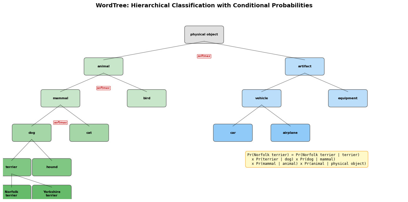
ax.set_title('WordTree: Hierarchical Classification with Conditional Probabilities',
             fontsize=14, fontweight='bold', pad=15)

# Tree nodes: (x, y, label, color)
nodes = [
    (7, 6.2, 'physical object', '#E0E0E0'),
    (3.5, 5.0, 'animal', '#C8E6C9'),
    (10.5, 5.0, 'artifact', '#BBDEFB'),
    (2, 3.8, 'mammal', '#C8E6C9'),
    (5, 3.8, 'bird', '#C8E6C9'),
    (9, 3.8, 'vehicle', '#BBDEFB'),
    (12, 3.8, 'equipment', '#BBDEFB'),
    (1, 2.5, 'dog', '#A5D6A7'),
    (3, 2.5, 'cat', '#A5D6A7'),
    (8, 2.5, 'car', '#90CAF9'),
    (10, 2.5, 'airplane', '#90CAF9'),
    (0.3, 1.2, 'terrier', '#81C784'),
    (1.7, 1.2, 'hound', '#81C784'),
    (0.3, 0.2, 'Norfolk\nterrier', '#66BB6A'),
    (1.7, 0.2, 'Yorkshire\nterrier', '#66BB6A'),
]

# Draw nodes
for x, y, label, color in nodes:
    rect = patches.FancyBboxPatch((x - 0.6, y - 0.25), 1.2, 0.5,
                                  boxstyle='round,pad=0.08',
                                  facecolor=color, edgecolor='#555555', linewidth=1)
    ax.add_patch(rect)
    ax.text(x, y, label, ha='center', va='center', fontsize=8, fontweight='bold')

# Draw edges
edges = [
    (7, 5.95, 3.5, 5.25), (7, 5.95, 10.5, 5.25),  # physical object -> animal, artifact
    (3.5, 4.75, 2, 4.05), (3.5, 4.75, 5, 4.05),    # animal -> mammal, bird
    (10.5, 4.75, 9, 4.05), (10.5, 4.75, 12, 4.05),  # artifact -> vehicle, equipment
    (2, 3.55, 1, 2.75), (2, 3.55, 3, 2.75),          # mammal -> dog, cat
    (9, 3.55, 8, 2.75), (9, 3.55, 10, 2.75),        # vehicle -> car, airplane
    (1, 2.25, 0.3, 1.45), (1, 2.25, 1.7, 1.45),    # dog -> terrier, hound
    (0.3, 0.95, 0.3, 0.45), (0.3, 0.95, 1.7, 0.45),  # terrier -> Norfolk, Yorkshire
]
for x1, y1, x2, y2 in edges:
    ax.plot([x1, x2], [y1, y2], 'k-', linewidth=1, alpha=0.5)

# Softmax annotations
softmax_groups = [
    (3.5, 10.5, 5.0, 'softmax'),  # animal vs artifact
    (2, 5, 3.8, 'softmax'),        # mammal vs bird
    (1, 3, 2.5, 'softmax'),        # dog vs cat
]
for x1, x2, y, label in softmax_groups:
    mid = (x1 + x2) / 2
    ax.annotate(label, xy=(mid, y + 0.35), fontsize=7, color='#C62828',
                ha='center', fontweight='bold', style='italic',
                bbox=dict(boxstyle='round,pad=0.15', facecolor='#FFEBEE', edgecolor='#C62828', alpha=0.8))

# Probability computation
prob_text = (
    'Pr(Norfolk terrier) = Pr(Norfolk terrier | terrier)\n'
    '  x Pr(terrier | dog) x Pr(dog | mammal)\n'
    '  x Pr(mammal | animal) x Pr(animal | physical object)'
)
ax.text(8.5, 1.5, prob_text, fontsize=9, va='center',
        bbox=dict(boxstyle='round,pad=0.5', facecolor='#FFF9C4', edgecolor='#F9A825', alpha=0.9),
        family='monospace')

plt.tight_layout()
plt.show()

9.3 Dataset Combination and Joint Training

Dataset combination. Categories from both COCO (80 detection classes) and the top 9000 ImageNet classes are mapped to synsets in the WordTree, producing a combined tree with 9418 classes. COCO is oversampled at a 4:1 ratio to balance with ImageNet.

Joint training algorithm. During training, detection and classification images are mixed:

  • Detection images (from COCO): backpropagate the full YOLOv2 loss (coordinates, objectness, and classification)
  • Classification images (from ImageNet): backpropagate only the classification loss at the label’s level in the tree and above. For example, if the label is “dog”, no error is assigned to finer distinctions like “German Shepherd” vs. “Golden Retriever”.

YOLO9000 uses 3 priors (instead of 5) to limit output size.

9.4 YOLO9000 Results

  • 19.7 mAP overall on the ImageNet detection validation set
  • 16.0 mAP on the 156 classes that have no detection training data (only classification labels)
  • Learns animal species well (objectness predictions generalize from COCO animals)
  • Struggles with clothing and equipment (COCO lacks bounding boxes for these categories)
  • Detects 9000+ object categories in real-time
Category Type Example Performance Reason
Animals (strong) armadillo (61.7), tiger (61.0) High mAP Objectness generalizes from COCO
Clothing (weak) sunglasses (0.0), swimming trunks (0.0) Near-zero mAP COCO has no clothing bounding boxes

10. Summary: Evolution from YOLOv1 to YOLOv2

Show code
import pandas as pd

comparison = {
    'Aspect': [
        'Backbone',
        'Box prediction',
        'Anchor priors',
        'Location encoding',
        'Normalization',
        'Input resolution',
        'Classifier pretraining',
        'Fine-grained features',
        'Number of classes',
        'VOC 2007 mAP',
        'Speed',
    ],
    'YOLOv1': [
        'Custom GoogLeNet-inspired (24 conv)',
        'Fully connected layers, direct coordinates',
        'None (grid cells only)',
        'Direct x,y relative to grid cell',
        'None (uses dropout)',
        'Fixed 448x448',
        '224x224 only',
        'None',
        '~20 (VOC)',
        '63.4%',
        '45 FPS',
    ],
    'YOLOv2': [
        'Darknet-19 (19 conv, fewer FLOPs)',
        'Convolutional, anchor box offsets',
        'k-means clustered dimension priors (k=5)',
        'Sigmoid-constrained relative to grid cell',
        'Batch normalization (no dropout)',
        'Multi-scale {320..608}',
        '224x224, then fine-tuned at 448x448',
        'Passthrough layer (26x26 to 13x13)',
        '9000+ (via WordTree joint training)',
        '78.6%',
        '40-91 FPS (resolution-dependent)',
    ]
}
df_cmp = pd.DataFrame(comparison)
df_cmp.style.set_properties(**{'text-align': 'left'}).set_table_styles([
    {'selector': 'th', 'props': [('text-align', 'left'), ('font-weight', 'bold')]}
]).set_caption('YOLOv1 vs YOLOv2: Side-by-Side Comparison')
Table 7: YOLOv1 vs YOLOv2: Side-by-Side Comparison
  Aspect YOLOv1 YOLOv2
0 Backbone Custom GoogLeNet-inspired (24 conv) Darknet-19 (19 conv, fewer FLOPs)
1 Box prediction Fully connected layers, direct coordinates Convolutional, anchor box offsets
2 Anchor priors None (grid cells only) k-means clustered dimension priors (k=5)
3 Location encoding Direct x,y relative to grid cell Sigmoid-constrained relative to grid cell
4 Normalization None (uses dropout) Batch normalization (no dropout)
5 Input resolution Fixed 448x448 Multi-scale {320..608}
6 Classifier pretraining 224x224 only 224x224, then fine-tuned at 448x448
7 Fine-grained features None Passthrough layer (26x26 to 13x13)
8 Number of classes ~20 (VOC) 9000+ (via WordTree joint training)
9 VOC 2007 mAP 63.4% 78.6%
10 Speed 45 FPS 40-91 FPS (resolution-dependent)

Key Themes

Several themes run through the evolution from YOLOv1 to YOLOv2:

  1. Detection as regression: Both papers maintain the core insight that detection can be cast as a single regression problem, avoiding the overhead of proposal generation.

  2. Speed/accuracy tradeoff: YOLOv1 prioritized speed with an acceptable accuracy gap. YOLOv2 closed the accuracy gap while maintaining speed, and introduced multi-scale inference for flexible tradeoffs at test time.

  3. Simplicity of architecture: Each improvement in v2 is motivated by a specific v1 limitation. The single-network, end-to-end pipeline is preserved throughout.

  4. Learned priors over hand-designed components: From hand-picked anchor boxes to k-means clustered dimension priors, from flat classification to hierarchical WordTree prediction — the trend is toward letting data drive design decisions.

  5. Bridging detection and classification: YOLO9000 demonstrated that hierarchical label spaces can bridge the gap between richly-labeled classification datasets and sparsely-labeled detection datasets, enabling detection of thousands of categories with minimal detection annotations.

The YOLO family established a research trajectory that continues to influence modern detection systems, with YOLOv3 and beyond building directly on the foundations laid in these two papers.

References

  1. Redmon, J., Divvala, S., Girshick, R., and Farhadi, A., “You Only Look Once: Unified, Real-Time Object Detection,” CVPR 2016.
  2. Redmon, J. and Farhadi, A., “YOLO9000: Better, Faster, Stronger,” CVPR 2017.