SSD: Single Shot MultiBox Detector

A technical walkthrough of SSD, the first real-time single-shot object detector to achieve over 70% mAP, combining multi-scale feature maps with convolutional predictors and default boxes.

Introduction and Motivation

By 2015, the dominant approach to object detection followed a two-stage pipeline: first generate region proposals, then classify each proposal with a convolutional network. Faster R-CNN represented the state of the art in this paradigm, achieving 73.2% mAP on PASCAL VOC2007 — but at only 7 frames per second (FPS). On the other end of the spectrum, YOLO (You Only Look Once) offered real-time speed at 45 FPS, but sacrificed accuracy significantly, reaching only 63.4% mAP.

The SSD paper by Liu et al. posed a direct question: can we build a detector that is both fast and accurate? Their answer was yes. SSD achieved 74.3% mAP at 59 FPS on VOC2007 — faster than YOLO and more accurate than Faster R-CNN.

The key insight was to eliminate the proposal generation step entirely and instead predict object categories and bounding box offsets directly from multiple feature maps at different scales, using small convolutional filters. This single-shot approach encapsulates all computation in one network, making it simple to train and deploy.

Method	mAP (VOC2007)	FPS	Input Size
Faster R-CNN (VGG16)	73.2%	7	~1000x600
YOLO (VGG16)	66.4%	21	448x448
SSD300	74.3%	59	300x300
SSD512	76.8%	22	512x512

SSD Architecture

The SSD architecture consists of three main components: a base network for feature extraction, multi-scale feature maps for detection at different resolutions, and convolutional predictors with default boxes at each feature map location.

Base Network: Truncated VGG-16

SSD uses VGG-16 (pre-trained on ImageNet) as its base network, but with several modifications:

1. The network is truncated after Conv5_3 — the fully connected classification layers are removed.
2. The original fc6 and fc7 layers are converted into convolutional layers (Conv6 and Conv7), with parameters subsampled from the original fully connected weights.
3. The pool5 layer is changed from \(2 \times 2\) stride-2 to \(3 \times 3\) stride-1.
4. Atrous (dilated) convolution is used in Conv6 to fill the “holes” introduced by the modified pooling, following the DeepLab-LargeFOV approach. This makes the network approximately 20% faster with no loss in accuracy compared to using the full VGG-16 without subsampling.
5. All dropout layers and the fc8 layer are removed.

Multi-Scale Feature Maps

After the base network, SSD adds extra convolutional layers that progressively decrease in spatial resolution. These layers form a feature pyramid that naturally handles objects of different sizes:

Feature Map	Spatial Size	Source
Conv4_3	38 x 38	From base VGG-16
Conv7 (FC7)	19 x 19	Converted FC layer
Conv8_2	10 x 10	Extra layer
Conv9_2	5 x 5	Extra layer
Conv10_2	3 x 3	Extra layer
Conv11_2	1 x 1	Extra layer

The intuition is straightforward: large feature maps (e.g., 38x38) have high spatial resolution and are better suited for detecting small objects, while small feature maps (e.g., 1x1) have large receptive fields and capture large objects.

This is fundamentally different from YOLO, which makes predictions from only a single feature map (7x7), and from Faster R-CNN, which applies the Region Proposal Network at a single scale.

Convolutional Predictors

At each feature map location, SSD applies \(3 \times 3\) convolutional filters to predict detections. For a feature layer of size \(m \times n\) with \(p\) channels, these small kernels produce:

• Class scores: \(c\) values (one per object category, including background)
• Box offsets: 4 values (\(\Delta cx, \Delta cy, \Delta w, \Delta h\)) relative to a default box

For \(k\) default boxes per location, this yields a total of \((c + 4) \times k\) filters per location, producing \((c + 4) \times k \times m \times n\) outputs for the entire feature map.

This convolutional approach is more parameter-efficient than YOLO’s fully connected layers and naturally preserves spatial structure.

Default Boxes and Aspect Ratios

At each feature map cell, SSD places a set of default bounding boxes (similar to Faster R-CNN’s anchors, but applied across multiple feature maps). The design of these boxes involves two parameters: scale and aspect ratio.

Scale formula. For \(m\) feature maps used for prediction, the scale at layer \(k\) is:

\[s_k = s_{\min} + \frac{s_{\max} - s_{\min}}{m - 1}(k - 1), \quad k \in [1, m]\]

where \(s_{\min} = 0.2\) and \(s_{\max} = 0.9\). The lowest layer detects objects at 20% of the image size, and the highest at 90%.

Aspect ratios. For each default box, the aspect ratios are drawn from \(a_r \in \{1, 2, 3, \tfrac{1}{2}, \tfrac{1}{3}\}\). The width and height are computed as:

\[w_k^a = s_k \sqrt{a_r}, \qquad h_k^a = s_k / \sqrt{a_r}\]

For the aspect ratio of 1, an additional default box with scale \(s_k' = \sqrt{s_k \cdot s_{k+1}}\) is added, resulting in 6 default boxes per location (for layers using all aspect ratios). Some layers (Conv4_3, Conv10_2, Conv11_2) use only 4 default boxes, omitting the \(\tfrac{1}{3}\) and \(3\) ratios.

The center of each default box is placed at \(\left(\frac{i + 0.5}{|f_k|}, \frac{j + 0.5}{|f_k|}\right)\), where \(|f_k|\) is the feature map size.

In total, SSD300 generates 8,732 default boxes across all six feature maps.

import numpy as np
import matplotlib.pyplot as plt
import matplotlib.patches as patches

# SSD300 default box scale computation
m = 6         # number of feature maps used for prediction
s_min = 0.2
s_max = 0.9

feature_maps = ['Conv4_3', 'Conv7', 'Conv8_2', 'Conv9_2', 'Conv10_2', 'Conv11_2']
fm_sizes     = [38, 19, 10, 5, 3, 1]
n_boxes      = [4, 6, 6, 6, 4, 4]  # default boxes per location

# Conv4_3 uses a special scale of 0.1; the formula applies to layers 2-6
scales = [0.1]  # Conv4_3 special scale
for k in range(1, m):
    s_k = s_min + (s_max - s_min) / (m - 1) * k
    scales.append(round(s_k, 2))

# Total default boxes
total_boxes = sum(fm**2 * nb for fm, nb in zip(fm_sizes, n_boxes))

print("SSD300 Feature Map Configuration")
print("=" * 65)
print(f"{'Layer':<12} {'Size':>6} {'Scale':>7} {'#Boxes/loc':>12} {'Total Boxes':>13}")
print("-" * 65)
for name, sz, sc, nb in zip(feature_maps, fm_sizes, scales, n_boxes):
    print(f"{name:<12} {sz:>4}x{sz:<4} {sc:>5.2f}   {nb:>8}       {sz*sz*nb:>6}")
print("-" * 65)
print(f"{'Total':<12} {'':>6} {'':>7} {'':>12} {total_boxes:>9}")

SSD300 Feature Map Configuration
=================================================================
Layer          Size   Scale   #Boxes/loc   Total Boxes
-----------------------------------------------------------------
Conv4_3        38x38    0.10          4         5776
Conv7          19x19    0.34          6         2166
Conv8_2        10x10    0.48          6          600
Conv9_2         5x5     0.62          6          150
Conv10_2        3x3     0.76          4           36
Conv11_2        1x1     0.90          4            4
-----------------------------------------------------------------
Total                                         8732

# Visualize default boxes at a single feature map location
fig, axes = plt.subplots(1, 3, figsize=(15, 5))

aspect_ratios_full = [1, 2, 3, 1/2, 1/3]  # plus extra box for ar=1
aspect_ratios_reduced = [1, 2, 1/2]        # plus extra box for ar=1

def draw_default_boxes(ax, scale, scale_next, aspect_ratios, title, include_extra=True):
    """Draw default boxes centered at (0.5, 0.5) on a unit square."""
    ax.set_xlim(0, 1)
    ax.set_ylim(0, 1)
    ax.set_aspect('equal')
    ax.set_title(title, fontsize=12, fontweight='bold')
    ax.add_patch(patches.Rectangle((0, 0), 1, 1, linewidth=1,
                                    edgecolor='gray', facecolor='#f0f0f0'))
    cx, cy = 0.5, 0.5
    colors = plt.cm.Set2(np.linspace(0, 1, 8))
    idx = 0
    labels = []
    for ar in aspect_ratios:
        w = scale * np.sqrt(ar)
        h = scale / np.sqrt(ar)
        rect = patches.Rectangle((cx - w/2, cy - h/2), w, h,
                                  linewidth=2, edgecolor=colors[idx],
                                  facecolor='none', linestyle='-')
        ax.add_patch(rect)
        labels.append(f'ar={ar:.1f}, s={scale:.1f}')
        idx += 1
    # Extra box for ar=1
    if include_extra:
        s_prime = np.sqrt(scale * scale_next)
        rect = patches.Rectangle((cx - s_prime/2, cy - s_prime/2), s_prime, s_prime,
                                  linewidth=2, edgecolor=colors[idx],
                                  facecolor='none', linestyle='--')
        ax.add_patch(rect)
        labels.append(f"ar=1, s'={s_prime:.2f}")
    ax.plot(cx, cy, 'r+', markersize=15, markeredgewidth=2)
    ax.legend(labels, loc='upper right', fontsize=7)

# Conv4_3: scale=0.1, 4 boxes (reduced aspect ratios)
draw_default_boxes(axes[0], 0.1, 0.2, aspect_ratios_reduced,
                   'Conv4_3 (38x38)\nScale=0.1, 4 boxes')

# Conv7: scale=0.34, 6 boxes (full aspect ratios)
draw_default_boxes(axes[1], 0.34, 0.48, aspect_ratios_full,
                   'Conv7 (19x19)\nScale=0.34, 6 boxes')

# Conv9_2: scale=0.62, 6 boxes
draw_default_boxes(axes[2], 0.62, 0.76, aspect_ratios_full,
                   'Conv9_2 (5x5)\nScale=0.62, 6 boxes')

plt.suptitle('Default Boxes at a Single Feature Map Location', fontsize=14, fontweight='bold', y=1.02)
plt.tight_layout()
plt.show()

Architecture Summary

The following diagram illustrates the full SSD300 pipeline. The key difference from YOLO is clear: SSD makes predictions from six feature maps at different resolutions, while YOLO uses only a single 7x7 feature map followed by fully connected layers.

fig, ax = plt.subplots(figsize=(16, 5))
ax.set_xlim(0, 16)
ax.set_ylim(0, 5)
ax.axis('off')
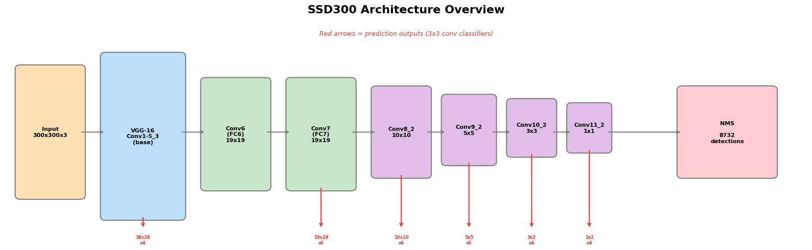
ax.set_title('SSD300 Architecture Overview', fontsize=16, fontweight='bold', pad=20)

# Define blocks: (x, y, width, height, label, color)
blocks = [
    (0.3, 1.0, 1.2, 3.0, 'Input\n300x300x3', '#FFE0B2'),
    (2.0, 0.5, 1.5, 3.8, 'VGG-16\nConv1-5_3\n(base)', '#BBDEFB'),
    (4.0, 1.2, 1.2, 2.5, 'Conv6\n(FC6)\n19x19', '#C8E6C9'),
    (5.7, 1.2, 1.2, 2.5, 'Conv7\n(FC7)\n19x19', '#C8E6C9'),
    (7.4, 1.5, 1.0, 2.0, 'Conv8_2\n10x10', '#E1BEE7'),
    (8.8, 1.8, 0.9, 1.5, 'Conv9_2\n5x5', '#E1BEE7'),
    (10.1, 2.0, 0.8, 1.2, 'Conv10_2\n3x3', '#E1BEE7'),
    (11.3, 2.1, 0.7, 1.0, 'Conv11_2\n1x1', '#E1BEE7'),
    (13.5, 1.5, 1.8, 2.0, 'NMS\n\n8732\ndetections', '#FFCDD2'),
]

for x, y, w, h, label, color in blocks:
    ax.add_patch(patches.FancyBboxPatch((x, y), w, h, boxstyle='round,pad=0.1',
                 facecolor=color, edgecolor='gray', linewidth=1.5))
    ax.text(x + w/2, y + h/2, label, ha='center', va='center', fontsize=8, fontweight='bold')

# Arrows between blocks
arrow_style = dict(arrowstyle='->', color='gray', lw=1.5)
connections = [
    (1.5, 2.5, 2.0, 2.5),
    (3.5, 2.5, 4.0, 2.5),
    (5.2, 2.5, 5.7, 2.5),
    (6.9, 2.5, 7.4, 2.5),
    (8.4, 2.5, 8.8, 2.5),
    (9.7, 2.5, 10.1, 2.5),
    (10.9, 2.5, 11.3, 2.5),
]
for x1, y1, x2, y2 in connections:
    ax.annotate('', xy=(x2, y2), xytext=(x1, y1), arrowprops=arrow_style)

# Prediction arrows (downward from detection layers)
pred_layers = [
    (2.75, 0.5, '38x38\nx4'),   # Conv4_3
    (6.3, 1.2, '19x19\nx6'),    # Conv7
    (7.9, 1.5, '10x10\nx6'),    # Conv8_2
    (9.25, 1.8, '5x5\nx6'),     # Conv9_2
    (10.5, 2.0, '3x3\nx4'),     # Conv10_2
    (11.65, 2.1, '1x1\nx4'),    # Conv11_2
]

for x, y_start, label in pred_layers:
    ax.annotate('', xy=(x, 0.2), xytext=(x, y_start),
                arrowprops=dict(arrowstyle='->', color='#E53935', lw=1.5))
    ax.text(x, 0.05, label, ha='center', va='top', fontsize=6, color='#E53935', fontweight='bold')

# Arrow from last pred layer area to NMS
ax.annotate('', xy=(13.5, 2.5), xytext=(12.0, 2.5),
            arrowprops=dict(arrowstyle='->', color='gray', lw=1.5))

ax.text(8.0, 4.8, 'Red arrows = prediction outputs (3x3 conv classifiers)', fontsize=9,
        ha='center', color='#E53935', style='italic')

plt.tight_layout()
plt.show()

Training Methodology

Training SSD requires assigning ground truth boxes to the fixed set of default boxes, then jointly optimizing localization and classification.

Matching Strategy

During training, SSD must determine which default boxes correspond to each ground truth object. The matching proceeds in two steps:

1. Best match: Each ground truth box is matched to the default box with the highest Jaccard overlap (IoU). This guarantees every ground truth has at least one matching default box.
2. Threshold match: Any default box with IoU > 0.5 to any ground truth is also matched.

This strategy simplifies learning by allowing multiple default boxes to be positive for a single ground truth, rather than forcing the network to pick only the best one.

Training Objective

The SSD loss function is a weighted sum of localization loss and confidence loss:

\[L(x, c, l, g) = \frac{1}{N}\left(L_{\text{conf}}(x, c) + \alpha \, L_{\text{loc}}(x, l, g)\right)\]

where \(N\) is the number of matched (positive) default boxes, and \(\alpha = 1\) (set by cross-validation).

Localization loss uses Smooth L1 loss between the predicted box (\(l\)) and the encoded ground truth (\(\hat{g}\)) over matched positive boxes:

\[L_{\text{loc}}(x, l, g) = \sum_{i \in \text{Pos}} \sum_{m \in \{cx, cy, w, h\}} x_{ij}^k \, \text{smooth}_{\text{L1}}(l_i^m - \hat{g}_j^m)\]

The ground truth offsets are encoded as:

\[\hat{g}_j^{cx} = \frac{g_j^{cx} - d_i^{cx}}{d_i^w}, \quad \hat{g}_j^{cy} = \frac{g_j^{cy} - d_i^{cy}}{d_i^h}, \quad \hat{g}_j^w = \log\frac{g_j^w}{d_i^w}, \quad \hat{g}_j^h = \log\frac{g_j^h}{d_i^h}\]

Confidence loss is the softmax cross-entropy over all classes:

\[L_{\text{conf}}(x, c) = -\sum_{i \in \text{Pos}} x_{ij}^p \log(\hat{c}_i^p) - \sum_{i \in \text{Neg}} \log(\hat{c}_i^0)\]

where \(\hat{c}_i^p = \frac{\exp(c_i^p)}{\sum_p \exp(c_i^p)}\) is the softmax probability.

Hard Negative Mining

With 8,732 default boxes and typically only a handful of positive matches per image, there is a severe class imbalance between positive and negative examples. Rather than using all negatives, SSD employs hard negative mining:

1. Sort all negative default boxes by their confidence loss (highest first).
2. Select the top negatives so that the ratio of negatives to positives is at most 3:1.

This focuses training on the most confusing negative examples and leads to faster convergence and more stable training.

Data Augmentation

Data augmentation is crucial for SSD — ablation studies show it contributes a +8.8% mAP improvement. Each training image is randomly processed by one of the following:

• Use the entire original image.
• Sample a random patch with minimum IoU of 0.1, 0.3, 0.5, 0.7, or 0.9 with existing objects.
• Sample a completely random patch.

Each sampled patch has a size between 10% and 100% of the original and an aspect ratio between \(\frac{1}{2}\) and 2. After sampling, the patch is resized to the fixed input size and horizontally flipped with probability 0.5, along with photometric distortions.

“Zoom Out” Augmentation for Small Objects

A follow-up “expansion” trick places the original image on a canvas 16x the original image area (filled with the dataset mean), before applying random crops. This “zoom out” operation effectively creates more small-object training examples and improves mAP by 2–3% across datasets. It is particularly effective for small objects, which are SSD’s main weakness.

Key Design Choices and Ablation Studies

The authors conduct careful ablation experiments (all on SSD300, VOC2007) to isolate the contribution of each design choice.

import matplotlib.pyplot as plt
import numpy as np

# Ablation study data from Table 2 of the paper
configs = [
    'Baseline\n(no aug, all boxes,\natrous)',
    '+ Data\nAugmentation',
    '+ {1/2, 2}\nAspect Ratios',
    '+ {1/3, 3}\nAspect Ratios',
    'Full SSD300\n(all components)',
]
mAP_values = [65.5, 71.6, 73.7, 74.2, 74.3]
increments = [0, 6.1, 2.1, 0.5, 0.1]

fig, ax = plt.subplots(figsize=(10, 5))
colors = ['#BBDEFB', '#90CAF9', '#64B5F6', '#42A5F5', '#1E88E5']
bars = ax.bar(range(len(configs)), mAP_values, color=colors, edgecolor='white', linewidth=1.5)

for bar, val, inc in zip(bars, mAP_values, increments):
    ax.text(bar.get_x() + bar.get_width()/2, bar.get_height() + 0.3,
            f'{val}%', ha='center', va='bottom', fontweight='bold', fontsize=11)
    if inc > 0:
        ax.text(bar.get_x() + bar.get_width()/2, bar.get_height() - 2,
                f'+{inc}%', ha='center', va='top', fontsize=9, color='white', fontweight='bold')

ax.set_xticks(range(len(configs)))
ax.set_xticklabels(configs, fontsize=9)
ax.set_ylabel('mAP (%)', fontsize=12)
ax.set_title('Ablation Study: Effect of Design Choices on SSD300 (VOC2007)', fontsize=13, fontweight='bold')
ax.set_ylim(60, 78)
ax.spines['top'].set_visible(False)
ax.spines['right'].set_visible(False)
plt.tight_layout()
plt.show()

Key Findings

Data augmentation is the single most important factor, contributing +8.8% mAP (from 65.5% baseline with only horizontal flip to 74.3% with the full augmentation strategy).

More default box shapes improve performance. Removing the \(\{\frac{1}{3}, 3\}\) aspect ratios drops mAP by 0.6%. Removing \(\{\frac{1}{2}, 2\}\) as well drops it by another 2.1%.

Atrous convolution is faster (~20%) with the same accuracy compared to using the full VGG-16 without subsampling.

Multi-Scale Prediction is Critical

The most important architectural contribution is the use of multiple output layers at different resolutions. The authors progressively remove prediction layers and show a monotonic decrease in accuracy:

# Multi-scale ablation data from Table 3
layers_used = [
    'Conv4_3 + Conv7 +\nConv8_2 + Conv9_2 +\nConv10_2 + Conv11_2',
    'Conv4_3 + Conv7 +\nConv8_2 + Conv9_2 +\nConv10_2',
    'Conv4_3 + Conv7 +\nConv8_2 + Conv9_2',
    'Conv4_3 + Conv7 +\nConv8_2',
    'Conv4_3 + Conv7',
    'Conv7 only',
]
n_layers = [6, 5, 4, 3, 2, 1]
mAP_multi = [74.3, 74.6, 73.8, 70.7, 64.2, 62.4]
n_boxes_multi = [8732, 8764, 8942, 9864, 9025, 8664]

fig, ax = plt.subplots(figsize=(9, 5))
colors_ml = plt.cm.RdYlGn(np.linspace(0.2, 0.9, len(n_layers)))
bars = ax.barh(range(len(layers_used)), mAP_multi, color=colors_ml[::-1], edgecolor='white', height=0.7)

for i, (bar, val, nb) in enumerate(zip(bars, mAP_multi, n_boxes_multi)):
    ax.text(bar.get_width() + 0.3, bar.get_y() + bar.get_height()/2,
            f'{val}% ({nb} boxes)', va='center', fontsize=10, fontweight='bold')

ax.set_yticks(range(len(layers_used)))
ax.set_yticklabels(layers_used, fontsize=8)
ax.set_xlabel('mAP (%)', fontsize=12)
ax.set_title('Effect of Multiple Output Layers (VOC2007 test)', fontsize=13, fontweight='bold')
ax.set_xlim(55, 82)
ax.invert_yaxis()
ax.spines['top'].set_visible(False)
ax.spines['right'].set_visible(False)
plt.tight_layout()
plt.show()

Reducing from 6 layers to a single layer drops performance from 74.3% to 62.4% — a loss of nearly 12 points. Even though the total number of boxes is kept roughly constant across configurations, concentrating all boxes at a single resolution is far less effective than distributing them across scales.

Experimental Results

SSD was evaluated on three major benchmarks: PASCAL VOC2007, PASCAL VOC2012, and MS COCO.

PASCAL VOC2007

The headline results on VOC2007 test demonstrate SSD’s speed-accuracy advantage:

Method	Training Data	mAP	FPS
Fast R-CNN	07+12	70.0%	-
Faster R-CNN	07+12	73.2%	7
YOLO (VGG16)	-	66.4%	21
SSD300	07+12	74.3%	59
SSD512	07+12	76.8%	22
SSD512	07+12+COCO	81.6%	22

SSD300 surpasses Faster R-CNN by 1.1% mAP while being over 8x faster. SSD512 extends the accuracy lead to 3.6%. With COCO pre-training, SSD512 reaches 81.6% mAP.

PASCAL VOC2012

On VOC2012 test, the same trend holds:

Method	Training Data	mAP
Faster R-CNN	07++12	70.4%
YOLO	07++12	57.9%
SSD300	07++12	72.4%
SSD512	07++12	74.9%
SSD512	07++12+COCO	80.0%

SSD512 outperforms Faster R-CNN by 4.5% mAP, and with COCO fine-tuning the gap widens to 4.1% over the COCO-pretrained Faster R-CNN.

MS COCO

On the more challenging COCO dataset (which emphasizes small objects), SSD512 achieves:

Method	mAP@[0.5:0.95]	mAP@0.5	mAP@0.75
Fast R-CNN	20.5	39.9	19.4
Faster R-CNN	24.2	45.3	23.5
SSD300	23.2	41.2	23.4
SSD512	26.8	46.5	27.8

SSD512 is 5.3% better in mAP@0.75 than Faster R-CNN, showing stronger localization quality. However, the improvement on small objects is more modest, as Faster R-CNN’s two-stage box refinement gives it an advantage for small objects.

# Speed vs. accuracy comparison
methods = ['Fast YOLO', 'YOLO (VGG16)', 'Faster R-CNN', 'SSD300', 'SSD512']
fps_vals = [155, 21, 7, 59, 22]
mAP_vals = [52.7, 66.4, 73.2, 74.3, 76.8]
colors_sa = ['#FFA726', '#FFA726', '#42A5F5', '#E53935', '#E53935']
markers = ['D', 'D', 's', 'o', 'o']

fig, ax = plt.subplots(figsize=(9, 6))

for name, fps, mAP, c, m in zip(methods, fps_vals, mAP_vals, colors_sa, markers):
    ax.scatter(fps, mAP, s=200, c=c, marker=m, edgecolors='black', linewidth=1, zorder=5)
    offset_x = 3 if fps < 100 else -10
    offset_y = 1.2
    if name == 'Faster R-CNN':
        offset_x = 2
        offset_y = -2.5
    elif name == 'SSD300':
        offset_y = -2.5
    ax.annotate(f'{name}\n({mAP}% mAP)', (fps, mAP),
                textcoords='offset points', xytext=(offset_x, offset_y),
                fontsize=9, fontweight='bold')

# Highlight the "real-time + accurate" region
ax.axhline(y=70, color='green', linestyle='--', alpha=0.3, linewidth=1.5)
ax.axvline(x=30, color='green', linestyle='--', alpha=0.3, linewidth=1.5)
ax.fill_between([30, 170], 70, 80, alpha=0.08, color='green')
ax.text(100, 78, 'Real-time + High Accuracy', ha='center', fontsize=10,
        color='green', style='italic', alpha=0.6)

ax.set_xlabel('Frames Per Second (FPS)', fontsize=12)
ax.set_ylabel('mAP (%) on VOC2007 test', fontsize=12)
ax.set_title('Speed vs. Accuracy Trade-off', fontsize=14, fontweight='bold')
ax.set_xlim(0, 170)
ax.set_ylim(48, 82)
ax.spines['top'].set_visible(False)
ax.spines['right'].set_visible(False)
ax.grid(True, alpha=0.2)
plt.tight_layout()
plt.show()

Weakness: Small Objects

Analysis of SSD’s detection performance by object size reveals a clear pattern: SSD is significantly worse on small objects compared to large ones. This is expected because small objects may not have sufficient information in the higher-level (coarser) feature maps.

The authors partially address this with:

• Larger input resolution (512x512 instead of 300x300)
• “Zoom out” data augmentation (placing images on a larger canvas), which creates more small-object training examples and boosts performance by 2–3% mAP

However, Faster R-CNN remains more competitive on small objects due to its two-step box refinement process (RPN + Fast R-CNN).

Comparison with Two-Stage Detectors and YOLO

Understanding where SSD sits relative to other detectors clarifies its contribution:

SSD vs. Faster R-CNN

Aspect	Faster R-CNN	SSD
Architecture	Two-stage (RPN + classifier)	Single-shot
Proposals	RPN generates ~6000 proposals	No proposals; 8732 default boxes
Feature resampling	RoI pooling per proposal	None
Prediction layers	Single feature map + FC layers	Multiple feature maps + conv filters
Anchor boxes	Single scale	Multiple scales across feature maps
Speed	~7 FPS	22–59 FPS
Small objects	Better (two refinement steps)	Weaker

SSD’s default boxes are conceptually similar to Faster R-CNN’s anchor boxes, but the key difference is that SSD applies them across multiple feature maps at different resolutions, naturally handling objects of various sizes without needing a proposal + pooling step.

SSD vs. YOLO

Aspect	YOLO	SSD
Feature maps	Single 7x7	Multiple (38x38 to 1x1)
Predictors	Fully connected layers	3x3 convolutional filters
Default boxes	2 boxes per cell, no aspect ratios	4–6 boxes per cell, multiple aspect ratios
Total predictions	98 per class	8732 per class
Input size	448x448	300x300 (faster, more accurate)
mAP (VOC2007)	63.4% (66.4% with VGG)	74.3%

SSD’s use of multiple feature maps and convolutional predictors with explicit aspect ratios accounts for its large accuracy advantage over YOLO.

Summary and Impact

SSD (Single Shot MultiBox Detector) introduced several ideas that became foundational in object detection:

1. Multi-scale feature maps for detection. By attaching convolutional predictors to feature maps at multiple resolutions, SSD efficiently handles objects of different sizes without image pyramids or proposal generation.

2. Convolutional predictors with default boxes. Small 3x3 convolutional filters predict class scores and box offsets for a fixed set of default boxes at each feature map location, combining the anchor box concept from Faster R-CNN with a fully convolutional single-shot design.

3. First real-time detector above 70% mAP. SSD300 achieved 74.3% mAP at 59 FPS, demonstrating that single-shot detection can match two-stage accuracy while being an order of magnitude faster.

4. Effective training strategies. Aggressive data augmentation (+8.8% mAP), hard negative mining (3:1 ratio), and the “zoom out” trick for small objects all proved essential for competitive performance.

The multi-scale feature map approach pioneered by SSD directly influenced later architectures like Feature Pyramid Networks (FPN) and became a standard component in modern detectors. SSD demonstrated that the two-stage detection paradigm was not inherently superior — with the right architectural choices and training strategies, a single-shot detector could achieve competitive accuracy at real-time speed.

---

This article is based on: Wei Liu, Dragomir Anguelov, Dumitru Erhan, Christian Szegedy, Scott Reed, Cheng-Yang Fu, Alexander C. Berg. “SSD: Single Shot MultiBox Detector.” ECCV 2016. arXiv:1512.02325.