Transformer Models

A survey of landmark transformer-based models — GPT, BERT, ViT, and T5 — covering their architectures, pre-training objectives, and downstream adaptation strategies including fine-tuning, zero-shot, one-shot, and few-shot inference.

NoneAbstract

This lesson surveys four landmark transformer-based architectures — GPT, BERT, ViT, and T5 — that have shaped modern deep learning. We examine how each model adapts the core transformer block (covered in the previous lesson) to different tasks and modalities: GPT uses decoder-only blocks with causal masking for autoregressive generation; BERT uses encoder-only blocks with bidirectional attention for language understanding; ViT applies the encoder architecture to image patches; and T5 employs the full encoder–decoder design with a text-to-text framework. We then compare downstream adaptation strategies: fine-tuning, zero-shot, one-shot, and few-shot inference. We follow Chapter 11 (D2L) notation throughout.

CREATED AT: 2026-03-05

Introduction

In the previous lesson we built the transformer architecture from the ground up: scaled dot-product attention, multi-head attention, the causal mask, positional encoding, residual connections, layer normalisation, and the feed-forward network. We assembled these into the transformer block and showed how blocks are stacked to form deep models.

With those building blocks in hand, we now turn to the transformer models that demonstrated the power of the transformer across different tasks and modalities. Each model makes a specific architectural choice — decoder-only, encoder-only, or encoder–decoder — and pairs it with a self-supervised pre-training objective that can leverage massive unlabelled corpora.

We conclude by discussing how pre-trained models are adapted to downstream tasks, contrasting traditional fine-tuning with the emergent capability of in-context learning.

Notation

We continue with Chapter 11 (D2L) notation:

Symbol	Meaning
\(n\)	Sequence length
\(d\)	Embedding dimension
\(L\)	Number of layers
\(h\)	Number of attention heads
\(\mathcal{V}\)	Vocabulary

The general transformer architecture

{image.png}

The general transformer consists of a encoder stack and a decoder stack, each can have one or more transformer blocks.

This architecture allows the most general sequence to sequence transformation. The input sequence, sources, is consumed by the encoder stack, using full-attention, producing a hidden sequence as the output of the encoder.

The output sequence, target, is generated autoregressively by the decoder block.

Part 1 — GPT: Decoder-Only Autoregressive Language Model

1.1 Architecture Overview

GPT uses decoder-only transformer blocks, each with a causally masked self-attention layer.

Input token sequence of length \(n\):

\[ \mathbf{x} = (x_1, x_2, \dots, x_n) \in \mathcal{V}^n. \]

Embedding (token + positional):

\[ \mathbf{X}^{(0)} = \mathbf{E}_{\text{token}} + \mathbf{E}_{\text{pos}} \in \mathbb{R}^{n \times d}. \]

Each of \(L\) decoder blocks applies masked multi-head self-attention then an FFN:

\[ \mathbf{X}^{(\ell)} = \operatorname{DecoderBlock}\!\left(\mathbf{X}^{(\ell-1)}\right), \quad \ell = 1, \dots, L. \]

The causal mask enforces:

\[ M_{ij} = \begin{cases} 0 & j \le i \\ -\infty & j > i. \end{cases} \]

Output logits over the vocabulary at each position:

\[ \mathbf{Z} = \mathbf{X}^{(L)} W_{\text{lm}}, \quad W_{\text{lm}} \in \mathbb{R}^{d \times |\mathcal{V}|}, \quad \mathbf{Z} \in \mathbb{R}^{n \times |\mathcal{V}|}. \]

The predicted probability of token \(x_t\) given its prefix:

\[ p(x_t \mid x_{<t}) = \operatorname{softmax}\!\left(\mathbf{Z}_{t-1}\right)_{x_t}. \]

image.png

import matplotlib.pyplot as plt
import matplotlib.patches as mpatches
import numpy as np

def draw_box(ax, xy, w, h, text, color="#4A90D9", fontsize=9, text_color="white"):
    rect = mpatches.FancyBboxPatch(xy, w, h, boxstyle="round,pad=0.06",
                                    facecolor=color, edgecolor="black", linewidth=1.2)
    ax.add_patch(rect)
    ax.text(xy[0] + w/2, xy[1] + h/2, text, ha="center", va="center",
            fontsize=fontsize, fontweight="bold", color=text_color)

def draw_arrow(ax, start, end):
    ax.annotate("", xy=end, xytext=start,
                arrowprops=dict(arrowstyle="-|>", color="black", lw=1.5))

# --- GPT Architecture Diagram ---
fig, ax = plt.subplots(figsize=(6, 7))
ax.set_xlim(-1, 7)
ax.set_ylim(-0.5, 9.5)
ax.set_aspect("equal")
ax.axis("off")
ax.set_title("GPT: Decoder-Only Architecture", fontsize=13, fontweight="bold", pad=10)

cx, bw = 1.5, 3.0

# Input tokens
ax.text(cx + bw/2, 0.0, r"Input tokens $(x_1, \ldots, x_n)$",
        ha="center", va="center", fontsize=10, fontweight="bold")

# Token + Positional Embedding
y = 0.8
draw_box(ax, (cx, y), bw, 0.6, "Token + Pos Embedding", color="#6C757D", fontsize=9)
draw_arrow(ax, (cx + bw/2, 0.25), (cx + bw/2, y))

# Decoder blocks
block_labels = ["Decoder Block 1\n(Masked Self-Attn + FFN)",
                "Decoder Block 2",
                "Decoder Block $L$"]
block_colors = ["#C0392B", "#C0392B", "#922B21"]
y_positions = [2.0, 3.3, 5.5]

draw_arrow(ax, (cx + bw/2, y + 0.6), (cx + bw/2, y_positions[0]))
for i, (yb, lbl, col) in enumerate(zip(y_positions, block_labels, block_colors)):
    draw_box(ax, (cx, yb), bw, 0.7, lbl, color=col, fontsize=8)
    if i == 1:
        draw_arrow(ax, (cx + bw/2, y_positions[0] + 0.7), (cx + bw/2, yb))
        # dots
        ax.text(cx + bw/2, yb + 0.7 + 0.4, "...", ha="center", va="center",
                fontsize=18, color="#555")
    if i == 2:
        draw_arrow(ax, (cx + bw/2, y_positions[1] + 0.7 + 0.7), (cx + bw/2, yb))

# Linear head
y_head = 6.8
draw_box(ax, (cx, y_head), bw, 0.6, r"Linear $W_{\rm lm}$", color="#8E44AD", fontsize=10)
draw_arrow(ax, (cx + bw/2, y_positions[2] + 0.7), (cx + bw/2, y_head))

# Softmax
y_sm = 7.9
draw_box(ax, (cx, y_sm), bw, 0.5, "Softmax", color="#27AE60", fontsize=10)
draw_arrow(ax, (cx + bw/2, y_head + 0.6), (cx + bw/2, y_sm))

# Output
ax.text(cx + bw/2, 8.8, r"$p(x_t \mid x_{<t})$",
        ha="center", va="center", fontsize=11, fontweight="bold")
draw_arrow(ax, (cx + bw/2, y_sm + 0.5), (cx + bw/2, 8.55))

# Annotation
ax.text(cx + bw + 0.4, 3.0, "Causal mask:\nupper triangle\n= $-\\infty$",
        fontsize=8, va="center", color="#C0392B", style="italic")

fig.tight_layout()
plt.show()

1.2 Autoregressive Token Generation (Inference)

At inference time, GPT generates one token at a time:

1. Start with a prompt \((x_1, \dots, x_k)\).
2. At step \(t \ge k+1\), feed the current sequence into the model.
3. Read logits at position \(t-1\):

\[ \hat{x}_t \sim \operatorname{softmax}\!\left(\mathbf{Z}_{t-1} / \tau\right), \]

where \(\tau\) is the temperature hyperparameter.

4. Append \(\hat{x}_t\) and repeat until an end-of-sequence token is produced or a length limit is reached.

ImportantKey Insight

Each generated token conditions on all previously generated tokens, but GPT never “looks ahead.” This is guaranteed by the causal mask.

import matplotlib.pyplot as plt
import numpy as np

def softmax(x, axis=-1):
    e = np.exp(x - np.max(x, axis=axis, keepdims=True))
    return e / e.sum(axis=axis, keepdims=True)

# --- Autoregressive generation: step-by-step visualisation ---
np.random.seed(7)
n = 8
d_k = 16
K_all = np.random.randn(n, d_k)
Q_all = np.random.randn(n, d_k)

fig, axes = plt.subplots(1, 4, figsize=(12, 3))
steps = [3, 5, 7, 8]  # how many tokens are "visible" at each step

for ax, t in zip(axes, steps):
    scores = Q_all[:t] @ K_all[:t].T / np.sqrt(d_k)
    mask = np.triu(np.full((t, t), -1e9), k=1)
    weights = softmax(scores + mask)
    im = ax.imshow(weights, cmap="Reds", vmin=0, vmax=weights.max())
    ax.set_title(f"Step t={t}", fontsize=10)
    ax.set_xlabel("Key pos")
    if t == steps[0]:
        ax.set_ylabel("Query pos")
    ax.set_xticks(range(t))
    ax.set_yticks(range(t))
    labels = [f"{i+1}" for i in range(t)]
    ax.set_xticklabels(labels, fontsize=7)
    ax.set_yticklabels(labels, fontsize=7)

fig.suptitle("GPT Autoregressive Generation: Causal Attention at Each Step",
             fontsize=12, fontweight="bold", y=1.04)
fig.tight_layout()
plt.show()

1.3 Training GPT: Next-Token Prediction

GPT is trained with the cross-entropy loss summed over every position:

\[ \mathcal{L}_{\text{GPT}} = -\frac{1}{n} \sum_{t=1}^{n} \log p_\theta(x_t \mid x_1, \dots, x_{t-1}). \]

Because the causal mask exposes all \(n-1\) prediction targets within a single forward pass, training is highly parallelisable despite the autoregressive nature of the model.

Training data. Large-scale web corpora (e.g., Common Crawl, Books). No manual labels are required — the raw text itself provides the supervision signal.

Scaling. GPT-2 (1.5 B parameters), GPT-3 (175 B parameters), and later GPT-4 demonstrate that scaling model size, dataset size, and compute jointly yields qualitatively richer language understanding. This empirical observation is sometimes called the scaling hypothesis.

---

Part 2 — BERT: Encoder-Only Masked Language Model

2.1 Architecture Overview

BERT uses encoder-only transformer blocks, each with full (bidirectional) self-attention — no causal mask.

Input tokens (after WordPiece tokenisation) of length \(n\):

\[ \mathbf{X}^{(0)} = \mathbf{E}_{\text{token}} + \mathbf{E}_{\text{pos}} + \mathbf{E}_{\text{seg}} \in \mathbb{R}^{n \times d}, \]

where \(\mathbf{E}_{\text{seg}}\) encodes which sentence a token belongs to (Segment A vs. Segment B).

Stacked encoder blocks:

\[ \mathbf{X}^{(\ell)} = \operatorname{EncoderBlock}\!\left(\mathbf{X}^{(\ell-1)}\right), \quad \ell = 1, \dots, L. \]

Output representations:

\[ \mathbf{H} = \mathbf{X}^{(L)} \in \mathbb{R}^{n \times d}. \]

A special [CLS] token is prepended; its final representation \(\mathbf{h}_{[\text{CLS}]} \in \mathbb{R}^d\) is used as a pooled sentence embedding for classification tasks.

image.png

import matplotlib.pyplot as plt
import matplotlib.patches as mpatches
import numpy as np

def draw_box(ax, xy, w, h, text, color="#4A90D9", fontsize=9, text_color="white"):
    rect = mpatches.FancyBboxPatch(xy, w, h, boxstyle="round,pad=0.06",
                                    facecolor=color, edgecolor="black", linewidth=1.2)
    ax.add_patch(rect)
    ax.text(xy[0] + w/2, xy[1] + h/2, text, ha="center", va="center",
            fontsize=fontsize, fontweight="bold", color=text_color)

def draw_arrow(ax, start, end):
    ax.annotate("", xy=end, xytext=start,
                arrowprops=dict(arrowstyle="-|>", color="black", lw=1.5))

# --- BERT vs GPT attention comparison ---
fig, axes = plt.subplots(1, 2, figsize=(9, 3.5))

n = 6
tokens = [f"$t_{{{i+1}}}$" for i in range(n)]

# GPT: causal mask
causal = np.tril(np.ones((n, n)))
axes[0].imshow(causal, cmap="Reds", vmin=0, vmax=1.5)
axes[0].set_title("GPT: Causal (Masked) Attention", fontsize=11)
axes[0].set_xlabel("Key position")
axes[0].set_ylabel("Query position")
axes[0].set_xticks(range(n)); axes[0].set_xticklabels(tokens)
axes[0].set_yticks(range(n)); axes[0].set_yticklabels(tokens)

# BERT: full attention
full = np.ones((n, n))
axes[1].imshow(full, cmap="Blues", vmin=0, vmax=1.5)
axes[1].set_title("BERT: Bidirectional (Full) Attention", fontsize=11)
axes[1].set_xlabel("Key position")
axes[1].set_ylabel("Query position")
axes[1].set_xticks(range(n)); axes[1].set_xticklabels(tokens)
axes[1].set_yticks(range(n)); axes[1].set_yticklabels(tokens)

fig.suptitle("GPT vs BERT: Attention Patterns", fontsize=13, fontweight="bold", y=1.02)
fig.tight_layout()
plt.show()

2.2 Pre-Training BERT: Masked Language Modelling (MLM)

BERT is pre-trained with two objectives.

Masked Language Modelling

Randomly mask 15% of input tokens. Of those:

• 80% are replaced with a special [MASK] token.
• 10% are replaced with a random token.
• 10% are left unchanged.

The model predicts the original token at each masked position \(\mathcal{M}\):

\[ \mathcal{L}_{\text{MLM}} = -\sum_{i \in \mathcal{M}} \log p_\theta\!\left(x_i \mid \tilde{\mathbf{x}}\right), \]

where \(\tilde{\mathbf{x}}\) is the corrupted sequence.

Because full self-attention is used, every masked token can attend to the entire context (left and right). This gives BERT deeply bidirectional representations.

Next Sentence Prediction (NSP)

Given a pair of sentences \(A\) and \(B\), predict whether \(B\) follows \(A\) in the original text:

\[ \mathcal{L}_{\text{NSP}} = -\log p_\theta\!\left(\text{IsNext} \mid \mathbf{h}_{[\text{CLS}]}\right). \]

ImportantGPT vs BERT

GPT uses masked (causal) self-attention, making it ideal for generation. BERT uses unmasked (bidirectional) self-attention, making it ideal for understanding tasks (classification, QA, named-entity recognition).

import matplotlib.pyplot as plt
import numpy as np

# --- Visualise BERT's MLM masking strategy ---
np.random.seed(42)

sentence = ["The", "cat", "sat", "on", "the", "mat", "today", "."]
n = len(sentence)

# Simulate 15% masking
mask_indices = [1, 5]  # 'cat' and 'mat' are masked
display = sentence.copy()
colors = ["#2ECC71"] * n  # green = unchanged

# 80% -> [MASK], 10% -> random, 10% -> unchanged
display[1] = "[MASK]"   # 80% case
colors[1] = "#E74C3C"   # red = [MASK]
display[5] = "dog"      # 10% random replacement
colors[5] = "#F39C12"   # orange = random

fig, ax = plt.subplots(figsize=(10, 2.5))
ax.set_xlim(-0.5, n - 0.5)
ax.set_ylim(-1, 3)
ax.axis("off")
ax.set_title("BERT MLM: Masking Strategy Example", fontsize=12, fontweight="bold")

# Original
ax.text(-0.5, 2.2, "Original:", fontsize=10, fontweight="bold", va="center")
for i, tok in enumerate(sentence):
    ax.text(i + 0.8, 2.2, tok, fontsize=11, ha="center", va="center",
            bbox=dict(boxstyle="round,pad=0.3", facecolor="#D5F5E3", edgecolor="#333"))

# Corrupted
ax.text(-0.5, 0.8, "Corrupted:", fontsize=10, fontweight="bold", va="center")
for i, (tok, col) in enumerate(zip(display, colors)):
    ax.text(i + 0.8, 0.8, tok, fontsize=11, ha="center", va="center",
            bbox=dict(boxstyle="round,pad=0.3", facecolor=col, edgecolor="#333",
                      alpha=0.3))

# Targets
ax.text(-0.5, -0.4, "Predict:", fontsize=10, fontweight="bold", va="center")
for i in mask_indices:
    ax.annotate(sentence[i], xy=(i + 0.8, 0.35), xytext=(i + 0.8, -0.4),
                fontsize=11, ha="center", va="center",
                arrowprops=dict(arrowstyle="-|>", color="#333", lw=1.2),
                bbox=dict(boxstyle="round,pad=0.3", facecolor="#AED6F1", edgecolor="#333"))

# Legend
legend_items = [
    plt.Line2D([0], [0], marker="s", color="w", markerfacecolor="#E74C3C", markersize=10, label="[MASK] (80%)"),
    plt.Line2D([0], [0], marker="s", color="w", markerfacecolor="#F39C12", markersize=10, label="Random (10%)"),
    plt.Line2D([0], [0], marker="s", color="w", markerfacecolor="#2ECC71", markersize=10, label="Unchanged (10%)"),
]
ax.legend(handles=legend_items, loc="upper right", fontsize=8, framealpha=0.9)

fig.tight_layout()
plt.show()

2.3 Key Design Choices

Property	GPT	BERT
Attention	Masked (causal)	Full (bidirectional)
Objective	Next-token prediction	MLM + NSP
Primary use	Generation	Understanding / classification
Output used	Last hidden state per position	[CLS] token or all tokens

---

Part 3 — Vision Transformer (ViT)

3.1 Motivation: Applying Transformers to Images

Transformers operate on sequences of vectors. Images are 2-D grids of pixels. ViT bridges this gap by converting an image into a sequence of patch embeddings, making images a first-class modality for transformer models.

image.png

3.2 Patch Tokenisation

Let the input image be:

\[ \mathbf{I} \in \mathbb{R}^{H \times W \times C}, \]

where \(H\) is height, \(W\) is width, and \(C\) is the number of channels.

Divide \(\mathbf{I}\) into a grid of non-overlapping patches of size \(P \times P\) pixels:

\[ N = \frac{H \times W}{P^2} \quad \text{patches.} \]

Each patch \(\mathbf{p}_i \in \mathbb{R}^{P^2 \cdot C}\) is flattened and projected to dimension \(d\):

\[ \mathbf{z}_i = \mathbf{p}_i W_E, \quad W_E \in \mathbb{R}^{(P^2 C) \times d}, \quad \mathbf{z}_i \in \mathbb{R}^d. \]

A learnable [CLS] token \(\mathbf{z}_0 \in \mathbb{R}^d\) is prepended. Learnable positional embeddings \(\mathbf{E}_{\text{pos}} \in \mathbb{R}^{(N+1) \times d}\) are added:

\[ \mathbf{X}^{(0)} = [\mathbf{z}_0;\, \mathbf{z}_1;\, \dots;\, \mathbf{z}_N] + \mathbf{E}_{\text{pos}} \in \mathbb{R}^{(N+1) \times d}. \]

import matplotlib.pyplot as plt
import matplotlib.patches as mpatches
import numpy as np

# --- ViT Patch Tokenisation Visualisation ---
fig, axes = plt.subplots(1, 3, figsize=(12, 4))

# 1. Original image (simulated as coloured grid)
H, W, P = 8, 8, 4  # 8x8 image, 4x4 patches -> 4 patches
np.random.seed(12)
img = np.random.rand(H, W, 3) * 0.5 + 0.3

axes[0].imshow(img)
axes[0].set_title(f"Input Image\n$H={H}, W={W}, C=3$", fontsize=10)
axes[0].set_xticks([])
axes[0].set_yticks([])

# 2. Image with patch grid
axes[1].imshow(img)
patch_colors = ["#E74C3C", "#3498DB", "#2ECC71", "#F39C12"]
N_patches = (H // P) * (W // P)
idx = 0
for r in range(0, H, P):
    for c in range(0, W, P):
        rect = mpatches.Rectangle((c - 0.5, r - 0.5), P, P,
                                   linewidth=2.5, edgecolor=patch_colors[idx % len(patch_colors)],
                                   facecolor="none")
        axes[1].add_patch(rect)
        axes[1].text(c + P/2 - 0.5, r + P/2 - 0.5, f"$p_{{{idx+1}}}$",
                     ha="center", va="center", fontsize=11, fontweight="bold",
                     color=patch_colors[idx % len(patch_colors)])
        idx += 1
axes[1].set_title(f"Patch Grid\n$P={P}, N={N_patches}$ patches", fontsize=10)
axes[1].set_xticks([])
axes[1].set_yticks([])

# 3. Resulting sequence
axes[2].set_xlim(-0.5, N_patches + 1.5)
axes[2].set_ylim(-1, 2)
axes[2].axis("off")
axes[2].set_title("Patch Embedding Sequence\n(input to Transformer)", fontsize=10)

# [CLS] token
axes[2].text(0, 0.5, "[CLS]", ha="center", va="center", fontsize=10, fontweight="bold",
             bbox=dict(boxstyle="round,pad=0.3", facecolor="#9B59B6", edgecolor="#333",
                       alpha=0.5))

# Patch tokens
for i in range(N_patches):
    axes[2].text(i + 1, 0.5, f"$z_{{{i+1}}}$", ha="center", va="center", fontsize=11,
                 fontweight="bold",
                 bbox=dict(boxstyle="round,pad=0.3",
                           facecolor=patch_colors[i % len(patch_colors)],
                           edgecolor="#333", alpha=0.4))

# + positional
axes[2].text((N_patches + 1) / 2, -0.4, r"$+ \mathbf{E}_{\rm pos}$",
             ha="center", va="center", fontsize=11, style="italic")

fig.suptitle("ViT: Image to Patch Embedding Sequence", fontsize=13, fontweight="bold", y=1.03)
fig.tight_layout()
plt.show()

3.3 Standard Transformer Encoder Applied to Patches

After tokenisation, the sequence \(\mathbf{X}^{(0)}\) is passed through \(L\) standard encoder blocks (full self-attention, no causal mask):

\[ \mathbf{X}^{(\ell)} = \operatorname{EncoderBlock}\!\left(\mathbf{X}^{(\ell-1)}\right), \quad \ell = 1, \dots, L. \]

The [CLS] token’s final representation is used for image classification:

\[ \hat{y} = \operatorname{softmax}\!\left(\mathbf{X}^{(L)}_0 \, W_{\text{cls}}\right). \]

3.4 Why ViT Works

Self-attention has global receptive field from the very first layer. Convolutions, by contrast, start local and build global context only gradually through depth. On large-scale pre-training data, ViT matches or exceeds convolutional networks.

ImportantKey Insight

ViT shows that the transformer is a domain-agnostic backbone: the same architecture, with a suitable tokenisation strategy, operates on text, images, audio, and more.

---

Part 4 — T5: Encoder–Decoder Text-to-Text Model

4.1 Architecture Overview

T5 is a full encoder–decoder transformer — the architecture introduced in the original “Attention is All You Need” paper.

Let the source sequence have length \(n_{\text{enc}}\) and the target sequence have length \(n_{\text{dec}}\).

Encoder (full self-attention):

\[ \mathbf{H}_{\text{enc}} = \operatorname{Encoder}\!\left(\mathbf{X}_{\text{enc}}\right) \in \mathbb{R}^{n_{\text{enc}} \times d}. \]

Decoder (masked self-attention + cross-attention to encoder):

\[ \mathbf{H}_{\text{dec}}^{(\ell)} = \operatorname{DecoderBlock}\!\left(\mathbf{H}_{\text{dec}}^{(\ell-1)},\, \mathbf{H}_{\text{enc}}\right). \]

Cross-attention at each decoder block:

\[ Q = \mathbf{H}_{\text{dec}}^{(\ell-1)} W_Q,\quad K = \mathbf{H}_{\text{enc}} W_K,\quad V = \mathbf{H}_{\text{enc}} W_V. \]

Output logits for the target sequence:

\[ \mathbf{Z} = \mathbf{H}_{\text{dec}}^{(L)} W_{\text{lm}} \in \mathbb{R}^{n_{\text{dec}} \times |\mathcal{V}|}. \]

image.png

import matplotlib.pyplot as plt
import matplotlib.patches as mpatches

def draw_box(ax, xy, w, h, text, color="#4A90D9", fontsize=9, text_color="white"):
    rect = mpatches.FancyBboxPatch(xy, w, h, boxstyle="round,pad=0.06",
                                    facecolor=color, edgecolor="black", linewidth=1.2)
    ax.add_patch(rect)
    ax.text(xy[0] + w/2, xy[1] + h/2, text, ha="center", va="center",
            fontsize=fontsize, fontweight="bold", color=text_color)

def draw_arrow(ax, start, end):
    ax.annotate("", xy=end, xytext=start,
                arrowprops=dict(arrowstyle="-|>", color="black", lw=1.5))

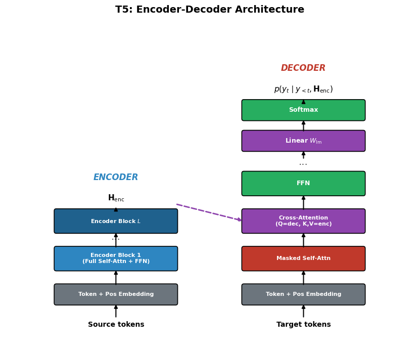
# --- T5 Encoder-Decoder Architecture ---
fig, ax = plt.subplots(figsize=(10, 7))
ax.set_xlim(-1, 11)
ax.set_ylim(-0.5, 9)
ax.set_aspect("equal")
ax.axis("off")
ax.set_title("T5: Encoder-Decoder Architecture", fontsize=14, fontweight="bold", pad=10)

# Encoder side
enc_x = 0.5
bw = 3.5

ax.text(enc_x + bw/2, 0.0, "Source tokens", ha="center", fontsize=10, fontweight="bold")
draw_box(ax, (enc_x, 0.7), bw, 0.5, "Token + Pos Embedding", color="#6C757D", fontsize=8)
draw_arrow(ax, (enc_x + bw/2, 0.25), (enc_x + bw/2, 0.7))

draw_box(ax, (enc_x, 1.7), bw, 0.6, "Encoder Block 1\n(Full Self-Attn + FFN)", color="#2E86C1", fontsize=8)
draw_arrow(ax, (enc_x + bw/2, 1.2), (enc_x + bw/2, 1.7))

draw_box(ax, (enc_x, 2.8), bw, 0.6, "Encoder Block $L$", color="#1F618D", fontsize=8)
ax.text(enc_x + bw/2, 2.55, "...", ha="center", fontsize=14, color="#555")
draw_arrow(ax, (enc_x + bw/2, 2.3), (enc_x + bw/2, 2.8))

ax.text(enc_x + bw/2, 3.7, r"$\mathbf{H}_{\rm enc}$", ha="center", fontsize=11, fontweight="bold")
draw_arrow(ax, (enc_x + bw/2, 3.4), (enc_x + bw/2, 3.55))

# Decoder side
dec_x = 6.0

ax.text(dec_x + bw/2, 0.0, "Target tokens", ha="center", fontsize=10, fontweight="bold")
draw_box(ax, (dec_x, 0.7), bw, 0.5, "Token + Pos Embedding", color="#6C757D", fontsize=8)
draw_arrow(ax, (dec_x + bw/2, 0.25), (dec_x + bw/2, 0.7))

draw_box(ax, (dec_x, 1.7), bw, 0.6, "Masked Self-Attn", color="#C0392B", fontsize=8)
draw_arrow(ax, (dec_x + bw/2, 1.2), (dec_x + bw/2, 1.7))

draw_box(ax, (dec_x, 2.8), bw, 0.6, "Cross-Attention\n(Q=dec, K,V=enc)", color="#8E44AD", fontsize=8)
draw_arrow(ax, (dec_x + bw/2, 2.3), (dec_x + bw/2, 2.8))

# Cross-attention arrow from encoder
ax.annotate("", xy=(dec_x, 3.1), xytext=(enc_x + bw, 3.6),
            arrowprops=dict(arrowstyle="-|>", color="#8E44AD", lw=2, ls="--"))

draw_box(ax, (dec_x, 3.9), bw, 0.6, "FFN", color="#27AE60", fontsize=9)
draw_arrow(ax, (dec_x + bw/2, 3.4), (dec_x + bw/2, 3.9))

ax.text(dec_x + bw/2, 4.75, "...", ha="center", fontsize=14, color="#555")

draw_box(ax, (dec_x, 5.2), bw, 0.5, r"Linear $W_{\rm lm}$", color="#8E44AD", fontsize=9)
draw_arrow(ax, (dec_x + bw/2, 4.9), (dec_x + bw/2, 5.2))

draw_box(ax, (dec_x, 6.1), bw, 0.5, "Softmax", color="#27AE60", fontsize=9)
draw_arrow(ax, (dec_x + bw/2, 5.7), (dec_x + bw/2, 6.1))

ax.text(dec_x + bw/2, 6.9, r"$p(y_t \mid y_{<t}, \mathbf{H}_{\rm enc})$",
        ha="center", fontsize=11, fontweight="bold")
draw_arrow(ax, (dec_x + bw/2, 6.6), (dec_x + bw/2, 6.7))

# Labels
ax.text(enc_x + bw/2, 4.3, "ENCODER", ha="center", fontsize=12,
        fontweight="bold", color="#2E86C1", style="italic")
ax.text(dec_x + bw/2, 7.5, "DECODER", ha="center", fontsize=12,
        fontweight="bold", color="#C0392B", style="italic")

fig.tight_layout()
plt.show()

4.2 The Text-to-Text Framework

The defining idea of T5: every NLP task is reformulated as mapping a text string to a text string.

Task	Input string	Target string
Translation	translate English to French: Hello	Bonjour
Summarisation	summarize: The cat sat on the ...	A cat sat.
Classification	sst2 sentence: This film is great	positive
Question answering	question: Who wrote Hamlet? context: ...	Shakespeare
Regression	stsb sentence1: A dog. sentence2: A cat.	3.8

A task-specific prefix in the input string signals to the model which task to perform.

NoteDefinition

Text-to-Text Framework: A unified formulation in which every NLP task — translation, summarisation, classification, question answering, regression — is expressed as a mapping from an input text string to an output text string. A task-specific prefix in the input selects the desired task.

4.3 Pre-Training T5: Span Corruption

T5 is pre-trained with a span corruption objective on the C4 (Colossal Clean Crawled Corpus) dataset.

Randomly select spans of tokens to mask. Replace each contiguous masked span with a single sentinel token \(\langle X \rangle\), \(\langle Y \rangle\), etc.:

\[ \text{Input:} \quad \text{"The} \underbrace{\text{ cat sat}}_{\langle X \rangle} \text{ on the} \underbrace{\text{ mat}}_{\langle Y \rangle} \text{."} \;\longrightarrow\; \text{"The} \langle X \rangle \text{on the} \langle Y \rangle \text{."} \]

The target is the concatenation of the masked spans labelled by their sentinels:

\[ \text{Target:} \quad \langle X \rangle \text{ cat sat} \langle Y \rangle \text{ mat} \langle Z \rangle. \]

Training loss (cross-entropy on target tokens only):

\[ \mathcal{L}_{\text{T5}} = -\sum_{t=1}^{n_{\text{dec}}} \log p_\theta\!\left(y_t \mid y_{<t},\, \mathbf{H}_{\text{enc}}\right). \]

ImportantComparison with BERT

Span corruption produces a much shorter target sequence than predicting every masked token independently, making training more efficient. T5 also generates the outputs autoregressively, which supports arbitrary-length text generation.

import matplotlib.pyplot as plt
import matplotlib.patches as mpatches

# --- T5 Span Corruption Visualisation ---
fig, ax = plt.subplots(figsize=(12, 4))
ax.set_xlim(-0.5, 12)
ax.set_ylim(-1.5, 4.5)
ax.axis("off")
ax.set_title("T5 Span Corruption: Pre-Training Objective", fontsize=13, fontweight="bold")

# Original sentence
original = ["The", "cat", "sat", "on", "the", "mat", "today", "."]
ax.text(-0.3, 3.5, "Original:", fontsize=10, fontweight="bold", va="center")
for i, tok in enumerate(original):
    color = "#D5F5E3"
    if i in [1, 2]:  # span 1
        color = "#FADBD8"
    elif i in [5]:   # span 2
        color = "#D6EAF8"
    ax.text(i + 1.2, 3.5, tok, ha="center", va="center", fontsize=11,
            bbox=dict(boxstyle="round,pad=0.25", facecolor=color, edgecolor="#333"))

# Encoder input (with sentinels)
enc_tokens = ["The", "<X>", "on", "the", "<Y>", "today", "."]
enc_colors = ["#D5F5E3", "#E74C3C", "#D5F5E3", "#D5F5E3", "#3498DB", "#D5F5E3", "#D5F5E3"]
ax.text(-0.3, 2.0, "Encoder\ninput:", fontsize=10, fontweight="bold", va="center")
for i, (tok, col) in enumerate(zip(enc_tokens, enc_colors)):
    tc = "white" if tok.startswith("<") else "black"
    ax.text(i + 1.2, 2.0, tok, ha="center", va="center", fontsize=11, color=tc,
            fontweight="bold" if tok.startswith("<") else "normal",
            bbox=dict(boxstyle="round,pad=0.25", facecolor=col if tok.startswith("<") else "#D5F5E3",
                      edgecolor="#333"))

# Decoder target
dec_tokens = ["<X>", "cat", "sat", "<Y>", "mat", "<Z>"]
dec_colors = ["#E74C3C", "#FADBD8", "#FADBD8", "#3498DB", "#D6EAF8", "#2ECC71"]
ax.text(-0.3, 0.5, "Decoder\ntarget:", fontsize=10, fontweight="bold", va="center")
for i, (tok, col) in enumerate(zip(dec_tokens, dec_colors)):
    tc = "white" if tok.startswith("<") else "black"
    ax.text(i + 1.2, 0.5, tok, ha="center", va="center", fontsize=11, color=tc,
            fontweight="bold" if tok.startswith("<") else "normal",
            bbox=dict(boxstyle="round,pad=0.25", facecolor=col, edgecolor="#333"))

# Braces for spans
ax.annotate("", xy=(2.2, 3.05), xytext=(3.2, 3.05),
            arrowprops=dict(arrowstyle="-", color="#E74C3C", lw=2))
ax.text(2.7, 2.85, "span 1", ha="center", fontsize=8, color="#E74C3C", style="italic")

fig.tight_layout()
plt.show()

4.4 Multi-Task Training

After pre-training, T5 is fine-tuned on a mixture of supervised tasks simultaneously. Each task contributes a proportion of the mini-batch. A task-specific prefix in the encoder input selects the task.

The combined loss is:

\[ \mathcal{L}_{\text{multi-task}} = \sum_{k} \lambda_k \, \mathcal{L}^{(k)}, \]

where \(\lambda_k\) is the mixing weight for task \(k\) and each \(\mathcal{L}^{(k)}\) is the cross-entropy loss on that task’s supervised data.

Benefits of multi-task training:

• Prevents overfitting on small datasets.
• Transfers knowledge across related tasks.
• Produces a single checkpoint that can handle many tasks at once.

---

Part 5 — Model Adaptation Strategies

Once a model has been pre-trained, several strategies exist for deploying it on downstream tasks. They differ in how much task-specific data is required and whether any model weights are updated.

5.1 Fine-Tuning

NoteDefinition

Fine-tuning: Given a pre-trained model with parameters \(\theta_{\text{pre}}\), continue gradient-based optimisation on a labelled task-specific dataset \(\mathcal{D} = \{(x_i, y_i)\}_{i=1}^{N}\).

\[ \theta^* = \arg\min_\theta \sum_{i=1}^{N} \mathcal{L}\!\left(f_\theta(x_i),\, y_i\right). \]

A lightweight classification or regression head \(W_{\text{head}}\) is typically added on top of the frozen or also-updated backbone.

Properties:

• Requires a labelled dataset (may be hundreds to millions of examples).
• Frequently achieves best task performance.
• Separate checkpoint per task.

5.2 In-Context Learning

NoteDefinition

In-context learning: The model weights are not updated. Instead, a carefully crafted prompt — the context — is placed in the input at inference time to guide the model’s output.

In-context learning is the primary adaptation paradigm for large autoregressive models such as GPT-3.

The context consists of a task description and, optionally, labelled demonstrations:

\[ \text{Prompt} = \underbrace{\text{[Task instruction]}}_{\text{optional}} \;\; \underbrace{(x_1, y_1), \dots, (x_k, y_k)}_{\text{k demonstrations}} \;\; \underbrace{x_{\text{query}}}_{\text{query}}. \]

The model returns \(\hat{y} = f_\theta(\text{Prompt})\) without any weight update.

The number of demonstrations \(k\) defines the shot regime.

5.3 Zero-Shot Inference (\(k = 0\))

No labelled examples are provided. Only a natural-language task description is given:

\[ \text{Prompt} = \text{"Translate English to French: Hello"} \]

The model must generalise from its pre-training distribution alone.

\[ \hat{y} = f_\theta(\text{task description} \;\|\; x_{\text{query}}). \]

Requirement: The task must be sufficiently represented in pre-training data for the model to understand it from the description alone.

5.4 One-Shot Inference (\(k = 1\))

One labelled \((x_1, y_1)\) demonstration is appended before the query:

\[ \text{Prompt} = \text{[description]} \;\|\; (x_1, y_1) \;\|\; x_{\text{query}}. \]

The single example illustrates the expected format and label space.

5.5 Few-Shot Inference (\(k \ge 2\))

Multiple demonstrations are provided:

\[ \text{Prompt} = \text{[description]} \;\|\; (x_1, y_1) \;\|\; \cdots \;\|\; (x_k, y_k) \;\|\; x_{\text{query}}. \]

More examples generally improve performance, subject to the model’s context window size. For GPT-3, \(k\) is practically limited to tens of examples due to the 2048-token context.

import matplotlib.pyplot as plt
import matplotlib.patches as mpatches

# --- Visualise Zero/One/Few-Shot Prompting ---
fig, axes = plt.subplots(3, 1, figsize=(11, 6), sharex=True)

def draw_prompt_block(ax, blocks, y=0.5, title=""):
    ax.set_xlim(-0.5, 12)
    ax.set_ylim(-0.2, 1.2)
    ax.axis("off")
    ax.set_title(title, fontsize=11, fontweight="bold", loc="left")
    x = 0
    for text, color, width in blocks:
        rect = mpatches.FancyBboxPatch((x, 0.15), width, 0.7,
                                        boxstyle="round,pad=0.08",
                                        facecolor=color, edgecolor="#333", linewidth=1)
        ax.add_patch(rect)
        ax.text(x + width/2, 0.5, text, ha="center", va="center",
                fontsize=8, fontweight="bold", color="white" if color != "#F9E79F" else "black")
        x += width + 0.15

# Zero-shot
draw_prompt_block(axes[0], [
    ("Task: Translate\nEnglish to French", "#2E86C1", 3.0),
    ("Hello", "#E67E22", 1.5),
    ("  -->  Bonjour", "#27AE60", 2.5),
], title="Zero-Shot ($k=0$): task description + query only")

# One-shot
draw_prompt_block(axes[1], [
    ("Task: Translate", "#2E86C1", 2.2),
    ("Good -> Bon", "#8E44AD", 2.2),
    ("Hello", "#E67E22", 1.5),
    ("  -->  Bonjour", "#27AE60", 2.5),
], title="One-Shot ($k=1$): task description + 1 example + query")

# Few-shot
draw_prompt_block(axes[2], [
    ("Task: Translate", "#2E86C1", 2.0),
    ("Good->Bon", "#8E44AD", 1.6),
    ("Cat->Chat", "#8E44AD", 1.6),
    ("Dog->Chien", "#8E44AD", 1.6),
    ("Hello", "#E67E22", 1.2),
    ("--> Bonjour", "#27AE60", 2.0),
], title="Few-Shot ($k=3$): task description + $k$ examples + query")

fig.suptitle("In-Context Learning: Prompt Structures", fontsize=13, fontweight="bold", y=1.02)
fig.tight_layout()
plt.show()

5.6 Comparison

Strategy	Labelled data needed	Weights updated	Separate checkpoint
Fine-tuning	Yes (many)	Yes	Yes
Zero-shot	No	No	No
One-shot	1 example	No	No
Few-shot	\(k\) examples (\(k \ll N\))	No	No

ImportantKey Insight

Large pre-trained models “store knowledge” in their weights. Zero/one/few-shot strategies access this stored knowledge through prompting alone, without gradient updates. Fine-tuning updates the weights to specialise the model, typically yielding better task performance when sufficient data is available.

---

Summary

Model	Architecture	Attention	Pre-training objective	Primary use
GPT	Decoder-only	Causal / masked	Next-token prediction	Generation
BERT	Encoder-only	Bidirectional	MLM + NSP	Understanding
ViT	Encoder-only	Bidirectional on patches	Supervised (ImageNet) / self-supervised	Vision
T5	Encoder–Decoder	Bidirectional (enc) + Causal (dec)	Span corruption + multi-task	Seq2seq / multi-task

References

1. Zhang, A., Lipton, Z. C., Li, M., & Smola, A. J., “Dive into Deep Learning, Chapter 11: Attention Mechanisms and Transformers”,