Introduction to Reinforcement Learning

An introduction to the foundations of reinforcement learning, covering Markov decision processes, value functions, Bellman equations, and tabular solution methods including dynamic programming, Monte Carlo, and temporal difference learning.

NoneAbstract

This lesson introduces the reinforcement learning (RL) framework, in which an agent learns to make sequential decisions by interacting with an environment to maximize cumulative reward. We build up from Markov processes to Markov reward processes and then to Markov decision processes (MDPs), which formalize the RL problem. We define state value functions and action value functions, derive the Bellman equations that express their recursive structure, and survey three families of tabular solution methods: dynamic programming, Monte Carlo methods, and temporal difference learning. The lesson concludes by discussing the limitations of tabular approaches and the motivation for function approximation.

CREATED AT: 2026-03-30

1. Foundations of Reinforcement Learning

Reinforcement learning (RL) is a sequential decision-making framework in which an agent learns to perform actions in an environment with the goal of maximizing received rewards. Unlike supervised learning, where a model is trained on labelled input-output pairs, RL agents must discover good behavior through trial and error — they receive only a scalar reward signal after taking actions, and must figure out which actions led to success.

Consider a concrete example: learning to play chess. An RL agent controls a character (the chess pieces), takes moves (actions), and receives a reward of \(+1\), \(-1\), or \(0\) at the end of the game depending on whether it wins, loses, or draws. This simple example already illustrates the core challenges of RL.

Core Challenges

1. Sparse rewards: The agent may need to play an entire game before receiving any feedback. There is no immediate signal telling the agent whether a particular move was good or bad.

2. Temporal credit assignment: A decisive advantage might be gained thirty moves before victory. The agent must learn to associate the reward at the end of the game with the critical action that occurred much earlier.

3. Stochastic environments: The opponent does not always make the same move in the same situation, so it is hard to know if an action was truly good or just lucky.

4. Exploration vs. exploitation: The agent must balance exploring the environment (trying new opening moves) with exploiting what it already knows (sticking to a previously successful opening). This is termed the exploration-exploitation trade-off.

import matplotlib.pyplot as plt
import matplotlib.patches as mpatches
import numpy as np

# Illustration: the agent-environment interaction loop
fig, ax = plt.subplots(1, 1, figsize=(7, 3.5))
ax.set_xlim(0, 10)
ax.set_ylim(0, 6)
ax.axis('off')

# Agent box
agent_box = mpatches.FancyBboxPatch((1, 3.5), 2.5, 1.5, boxstyle='round,pad=0.2',
                                     facecolor='#4C72B0', edgecolor='black', linewidth=1.5)
ax.add_patch(agent_box)
ax.text(2.25, 4.25, 'Agent\n$\\pi(a_t | s_t)$', ha='center', va='center',
        fontsize=11, color='white', fontweight='bold')

# Environment box
env_box = mpatches.FancyBboxPatch((5.5, 3.5), 3, 1.5, boxstyle='round,pad=0.2',
                                   facecolor='#55A868', edgecolor='black', linewidth=1.5)
ax.add_patch(env_box)
ax.text(7, 4.25, 'Environment\n$P(s_{t+1}|s_t,a_t)$', ha='center', va='center',
        fontsize=11, color='white', fontweight='bold')

# Action arrow (agent -> environment)
ax.annotate('', xy=(5.5, 4.8), xytext=(3.5, 4.8),
            arrowprops=dict(arrowstyle='->', lw=2, color='#C44E52'))
ax.text(4.5, 5.2, 'action $a_t$', ha='center', va='center', fontsize=10, color='#C44E52')

# State arrow (environment -> agent, bottom)
ax.annotate('', xy=(3.5, 3.7), xytext=(5.5, 3.7),
            arrowprops=dict(arrowstyle='->', lw=2, color='#8172B2'))
ax.text(4.5, 3.0, 'state $s_{t+1}$, reward $r_{t+1}$', ha='center', va='center',
        fontsize=10, color='#8172B2')

ax.set_title('The Reinforcement Learning Loop', fontsize=13, fontweight='bold', pad=15)
plt.tight_layout()
plt.show()

The diagram above captures the essence of RL: at each time step \(t\), the agent observes the current state \(s_t\), selects an action \(a_t\) according to its policy \(\pi(a_t | s_t)\), and the environment responds with a new state \(s_{t+1}\) and a reward \(r_{t+1}\). The cycle then repeats.

---

2. From Markov Processes to Markov Reward Processes

To formalize the RL problem, we build up through a sequence of increasingly rich mathematical models.

2.1 Markov Process (MP)

A Markov process assumes that the world is always in one of a set of possible states. The key property — the Markov property — states that the probability of transitioning to the next state depends only on the current state and not on the history of states that preceded it.

ImportantMarkov Process

A Markov process is defined by:

• A finite set of states \(\mathcal{S} = \{s_1, s_2, \ldots, s_n\}\)
• Transition probabilities \(P(s_{t+1} \mid s_t)\) specifying the probability of moving to state \(s_{t+1}\) given the current state \(s_t\)

The Markov property: \(P(s_{t+1} \mid s_1, s_2, \ldots, s_t) = P(s_{t+1} \mid s_t)\).

The Markov property is a memorylessness assumption: the future is conditionally independent of the past given the present. This simplification is what makes the mathematical framework tractable.

The process produces a sequence (trajectory) of states \(\tau = [s_1, s_2, s_3, \ldots]\) as the system evolves over time.

Consider the textbook’s penguin-on-ice example: a penguin can visit 16 different positions on a 4x4 grid. Because the ice is slippery, at each time step the penguin has an equal probability of moving to any adjacent state. For example, in position 6, it has a 25% chance of moving to states 2, 5, 7, or 10.

# Visualize a simple 4x4 Markov process transition matrix (slippery ice grid)
# States numbered 1-16 in row-major order on a 4x4 grid

def get_neighbors(state, rows=4, cols=4):
    """Get neighboring states for a grid position (1-indexed)."""
    r, c = divmod(state - 1, cols)
    neighbors = []
    for dr, dc in [(-1, 0), (1, 0), (0, -1), (0, 1)]:
        nr, nc = r + dr, c + dc
        if 0 <= nr < rows and 0 <= nc < cols:
            neighbors.append(nr * cols + nc + 1)
    return neighbors

n_states = 16
P = np.zeros((n_states, n_states))
for s in range(1, n_states + 1):
    nbrs = get_neighbors(s)
    for nb in nbrs:
        P[s - 1, nb - 1] = 1.0 / len(nbrs)

fig, axes = plt.subplots(1, 2, figsize=(11, 4.5))

# Left: the grid
ax = axes[0]
ax.set_xlim(-0.5, 3.5)
ax.set_ylim(-0.5, 3.5)
ax.set_aspect('equal')
ax.invert_yaxis()
for i in range(4):
    for j in range(4):
        state = i * 4 + j + 1
        rect = plt.Rectangle((j - 0.5, i - 0.5), 1, 1, fill=True,
                              facecolor='#d6eaf8', edgecolor='#2c3e50', linewidth=1.5)
        ax.add_patch(rect)
        ax.text(j, i, str(state), ha='center', va='center', fontsize=12, fontweight='bold')
ax.set_xticks([])
ax.set_yticks([])
ax.set_title('4x4 Grid World (State Labels)', fontsize=12, fontweight='bold')

# Right: transition matrix heatmap
ax = axes[1]
im = ax.imshow(P, cmap='Blues', vmin=0, vmax=0.5)
ax.set_xlabel('Next state $s_{t+1}$', fontsize=11)
ax.set_ylabel('Current state $s_t$', fontsize=11)
ax.set_title('Transition Matrix $P(s_{t+1} | s_t)$', fontsize=12, fontweight='bold')
ax.set_xticks(range(0, 16, 2))
ax.set_xticklabels(range(1, 17, 2))
ax.set_yticks(range(0, 16, 2))
ax.set_yticklabels(range(1, 17, 2))
plt.colorbar(im, ax=ax, shrink=0.8)

plt.tight_layout()
plt.show()

2.2 Markov Reward Process (MRP)

A Markov reward process extends the Markov process by associating a reward distribution \(P(r_{t+1} \mid s_t)\) with each state. When the system is in state \(s_t\) and transitions, it also emits a reward \(r_{t+1}\).

ImportantThe Return

The MRP introduces a discount factor \(\gamma \in (0, 1]\) and defines the return \(G_t\) — the cumulative discounted future reward from time \(t\) onward:

\[ G_t = \sum_{k=0}^{\infty} \gamma^k \, r_{t+k+1}. \]

A discount factor \(\gamma < 1\) makes rewards closer in time more valuable. This is both mathematically convenient (ensures the sum converges for bounded rewards) and intuitively reasonable (an immediate reward is generally preferred over a delayed one).

The return measures the total future benefit of being on a particular trajectory.

In the penguin example, the rewards are deterministic: the penguin receives \(+1\) if it lands on a fish, and \(0\) otherwise. With \(\gamma = 0.9\), the return grows as the penguin gets closer to the fish.

# Illustrate how the return G_t changes with the discount factor gamma

gammas = [0.5, 0.7, 0.9, 0.99]
# Example: rewards arrive at steps 3, 7, and 10 (each +1)
T = 15
reward_steps = [3, 7, 10]
rewards = np.zeros(T)
for step in reward_steps:
    rewards[step] = 1.0

fig, axes = plt.subplots(1, 2, figsize=(12, 4))

# Left: discount weights over time for different gamma
ax = axes[0]
steps = np.arange(T)
for gamma in gammas:
    weights = gamma ** steps
    ax.plot(steps, weights, 'o-', markersize=4, label=f'$\\gamma = {gamma}$')
ax.set_xlabel('Time step $k$', fontsize=11)
ax.set_ylabel('Discount weight $\\gamma^k$', fontsize=11)
ax.set_title('Discount Weights Over Time', fontsize=12, fontweight='bold')
ax.legend(fontsize=9)
ax.grid(True, alpha=0.3)

# Right: return G_t for different gamma
ax = axes[1]
for gamma in gammas:
    G = np.zeros(T)
    for t in range(T):
        for k in range(t, T):
            G[t] += (gamma ** (k - t)) * rewards[k]
    ax.plot(steps, G, 'o-', markersize=4, label=f'$\\gamma = {gamma}$')
# Mark reward steps
for rs in reward_steps:
    ax.axvline(x=rs, color='gray', linestyle='--', alpha=0.4)
ax.set_xlabel('Time step $t$', fontsize=11)
ax.set_ylabel('Return $G_t$', fontsize=11)
ax.set_title('Return $G_t$ (rewards at steps 3, 7, 10)', fontsize=12, fontweight='bold')
ax.legend(fontsize=9)
ax.grid(True, alpha=0.3)

plt.tight_layout()
plt.show()

The left panel shows how the discount factor controls the weight placed on future rewards. When \(\gamma\) is small, only the immediate next few rewards matter. When \(\gamma\) is close to 1, the agent is far-sighted and cares about rewards far into the future.

The right panel shows the return \(G_t\) at each time step, given that rewards of \(+1\) arrive at steps 3, 7, and 10. Notice that the return is always highest just before a reward is received, and that larger \(\gamma\) values produce higher overall returns because the agent accounts for distant rewards.

---

3. Markov Decision Processes (MDP)

A Markov decision process extends the MRP by introducing actions. At each time step, the agent chooses an action \(a_t\) from a set of available actions, and this choice influences both the state transition and the reward.

3.1 MDP Components

ImportantMDP Definition

An MDP is defined by the tuple \((\mathcal{S}, \mathcal{A}, P, r, \gamma)\):

• States \(\mathcal{S}\): the set of all possible states \(s\)
• Actions \(\mathcal{A}\): the set of all possible actions \(a\)
• Transition probabilities \(P(s' \mid s, a)\): the probability of transitioning to state \(s'\) when taking action \(a\) in state \(s\)
• Rewards \(r(s, a)\): the reward received after taking action \(a\) in state \(s\)
• Discount factor \(\gamma \in (0, 1]\)

The MDP extends the MRP by introducing actions, giving the agent control over state transitions. This is the standard formalization of the RL problem.

A trajectory from an MDP consists of alternating states, actions, and rewards:

\[ (s_1, a_1, r_2, s_2, a_2, r_3, \ldots) \]

In the penguin example, the four actions correspond to moving up, right, down, and left. Because the ice is slippery, the penguin moves in the intended direction with only 50% probability and may slide to one of the other adjacent positions with equal probability.

3.2 POMDP (Brief Mention)

In a partially observable Markov decision process (POMDP), the agent does not directly observe the true state \(s_t\). Instead, it receives an observation \(o_t\) drawn from \(P(o_t \mid s_t)\). This makes the problem significantly harder, because the agent must maintain a belief over possible states. Most RL algorithms assume full observability (i.e., a standard MDP), but POMDPs are important in practice — for example, when the agent can only see a limited portion of its surroundings.

3.3 Policies

A policy \(\pi\) defines the agent’s behavior: it maps states to actions.

NoteTypes of Policies

• Deterministic policy: \(\pi(s)\) returns a single action for each state.
• Stochastic policy: \(\pi(a \mid s)\) returns a probability distribution over actions for each state.
• Stationary policy: depends only on the current state, not on the time step.
• Non-stationary policy: may change its behavior over time.

We use the notation \(\pi(a \mid s)\) for stochastic policies. A deterministic policy is a special case where \(\pi(a \mid s) = 1\) for exactly one action and \(0\) for all others.

# Visualize a deterministic policy on the 4x4 grid
# Actions: 0=up, 1=right, 2=down, 3=left
action_symbols = {'up': '\u2191', 'right': '\u2192', 'down': '\u2193', 'left': '\u2190'}
action_names = ['up', 'right', 'down', 'left']

# A simple policy that generally moves toward bottom-right (where a fish might be)
det_policy = [
    'right', 'right', 'down', 'down',
    'down',  'right', 'right', 'down',
    'right', 'down',  'right', 'down',
    'right', 'right', 'right', 'right',  # state 16 is the goal
]

# A stochastic policy with preferences
np.random.seed(42)
stoch_policy = np.random.dirichlet([1, 2, 2, 1], size=16)

fig, axes = plt.subplots(1, 2, figsize=(10, 4.5))

# Left: deterministic policy
ax = axes[0]
ax.set_xlim(-0.5, 3.5)
ax.set_ylim(-0.5, 3.5)
ax.set_aspect('equal')
ax.invert_yaxis()
for i in range(4):
    for j in range(4):
        state_idx = i * 4 + j
        color = '#abebc6' if state_idx == 15 else '#d6eaf8'
        rect = plt.Rectangle((j - 0.5, i - 0.5), 1, 1, fill=True,
                              facecolor=color, edgecolor='#2c3e50', linewidth=1.5)
        ax.add_patch(rect)
        arrow = action_symbols[det_policy[state_idx]]
        ax.text(j, i, arrow, ha='center', va='center', fontsize=18, fontweight='bold')
ax.set_xticks([])
ax.set_yticks([])
ax.set_title('Deterministic Policy', fontsize=12, fontweight='bold')

# Right: stochastic policy (show arrow sizes proportional to probability)
ax = axes[1]
ax.set_xlim(-0.5, 3.5)
ax.set_ylim(-0.5, 3.5)
ax.set_aspect('equal')
ax.invert_yaxis()
arrow_offsets = {'up': (0, -0.25), 'right': (0.25, 0), 'down': (0, 0.25), 'left': (-0.25, 0)}
for i in range(4):
    for j in range(4):
        state_idx = i * 4 + j
        color = '#abebc6' if state_idx == 15 else '#d6eaf8'
        rect = plt.Rectangle((j - 0.5, i - 0.5), 1, 1, fill=True,
                              facecolor=color, edgecolor='#2c3e50', linewidth=1.5)
        ax.add_patch(rect)
        for a_idx, a_name in enumerate(action_names):
            prob = stoch_policy[state_idx, a_idx]
            dx, dy = arrow_offsets[a_name]
            ax.annotate('', xy=(j + dx, i + dy), xytext=(j, i),
                        arrowprops=dict(arrowstyle='->', lw=1 + 3 * prob,
                                        color=plt.cm.Reds(0.3 + 0.7 * prob)))
ax.set_xticks([])
ax.set_yticks([])
ax.set_title('Stochastic Policy', fontsize=12, fontweight='bold')

plt.tight_layout()
plt.show()

The left panel shows a deterministic policy where each state maps to exactly one action (shown as an arrow). The right panel shows a stochastic policy where each state has a probability distribution over actions (thicker, darker arrows indicate higher probability). Stochastic policies have the advantage of encouraging exploration.

3.4 The RL Loop

The agent and environment interact in a loop:

1. The agent observes state \(s_t\)
2. The agent selects action \(a_t\) according to its policy \(\pi(a_t \mid s_t)\)
3. The environment transitions to a new state \(s_{t+1} \sim P(s_{t+1} \mid s_t, a_t)\)
4. The environment emits a reward \(r_{t+1} \sim P(r_{t+1} \mid s_t, a_t)\)
5. Repeat

The goal of RL is to find a policy \(\pi\) that maximizes the expected return over this interaction loop.

---

4. RL Objective: Expected Return

The goal of reinforcement learning is to find a policy \(\pi\) that maximizes the expected return. To make this precise, we define value functions that quantify how good it is to be in a given state (or to take a given action in a given state) under a particular policy.

4.1 State Value Function

ImportantState Value Function

The state value function \(v^\pi(s)\) gives the expected return starting from state \(s\) and following policy \(\pi\) thereafter:

\[ v^\pi(s) = \mathbb{E}\left[G_t \mid s_t = s\right]. \]

Informally, \(v^\pi(s)\) tells us the long-term reward we can expect on average if we start in state \(s\) and follow policy \(\pi\). It is highest for states where subsequent transitions will bring large rewards soon.

4.2 Action Value Function

ImportantAction Value Function

The action value function \(q^\pi(s, a)\) gives the expected return starting from state \(s\), taking action \(a\), and then following policy \(\pi\) thereafter:

\[ q^\pi(s, a) = \mathbb{E}\left[G_t \mid s_t = s, a_t = a\right]. \]

The action value connects future rewards to current actions, directly addressing the temporal credit assignment problem. It is the quantity most RL algorithms seek to estimate.

4.3 Optimal Values and Optimal Policy

ImportantOptimal Values and Policy

The optimal state value function \(v^*(s)\) and optimal action value function \(q^*(s, a)\) are obtained by maximizing over all possible policies:

\[ v^*(s) = \max_\pi \, v^\pi(s), \qquad q^*(s, a) = \max_\pi \, q^\pi(s, a). \]

The optimal policy is:

\[ \pi^*(s) = \arg\max_a \, q^*(s, a). \]

For MDPs (but not POMDPs), there always exists a deterministic, stationary policy that maximizes the value of every state. This is the core idea: estimate \(q^*\) and act greedily.

# Visualize state values on a 4x4 grid
# Reward of +1 at state 16 (bottom-right corner), gamma=0.9
# Simple approximate values: closer to the goal => higher value

gamma = 0.9
goal_r, goal_c = 3, 3  # state 16

# Approximate state values based on Manhattan distance
values_grid = np.zeros((4, 4))
for i in range(4):
    for j in range(4):
        dist = abs(i - goal_r) + abs(j - goal_c)
        values_grid[i, j] = gamma ** dist

fig, ax = plt.subplots(1, 1, figsize=(5, 4.5))
im = ax.imshow(values_grid, cmap='YlOrRd', vmin=0, vmax=1)
for i in range(4):
    for j in range(4):
        ax.text(j, i, f'{values_grid[i, j]:.2f}', ha='center', va='center',
                fontsize=13, fontweight='bold',
                color='white' if values_grid[i, j] > 0.6 else 'black')
ax.set_xticks(range(4))
ax.set_xticklabels([1, 2, 3, 4])
ax.set_yticks(range(4))
ax.set_yticklabels([1, 5, 9, 13])
ax.set_title('State Values $v^\\pi(s)$ (reward at state 16)', fontsize=12, fontweight='bold')
plt.colorbar(im, ax=ax, shrink=0.8, label='Value')

# Add a marker for the goal
ax.plot(3, 3, 's', color='lime', markersize=20, markeredgecolor='black', markeredgewidth=2)
ax.text(3, 3, 'G', ha='center', va='center', fontsize=10, fontweight='bold')

plt.tight_layout()
plt.show()

The figure above shows approximate state values on a 4x4 grid, where a reward of \(+1\) is located at the bottom-right corner (state 16, marked “G” for goal). States closer to the goal have higher values because the discounted reward \(\gamma^d\) decreases with Manhattan distance \(d\) from the goal. This is exactly the intuition: states from which the agent can quickly reach the reward are more valuable.

---

5. Bellman Equations

The Bellman equations express a fundamental recursive relationship between the value of a state (or state-action pair) and the values of its successor states. They are the mathematical backbone of nearly all RL algorithms.

5.1 Relating State Values and Action Values

ImportantState-Action Value Relationship

The state value \(v(s)\) can be expressed as a weighted sum of the action values \(q(s, a)\):

\[ v(s) = \sum_a \pi(a \mid s) \, q(s, a). \]

Conversely, the action value decomposes into immediate reward plus discounted future value:

\[ q(s, a) = r(s, a) + \gamma \sum_{s'} P(s' \mid s, a) \, v(s'). \]

The first equation says: the value of a state is the expected action value under the policy. The second says: the value of an action is the immediate reward plus the discounted expected value of wherever we end up.

5.2 Bellman Expectation Equation (Policy Evaluation)

ImportantBellman Expectation Equation

Substituting the action-value decomposition into the state-value equation, we get:

\[ v(s) = \sum_a \pi(a \mid s) \left[ r(s, a) + \gamma \sum_{s'} P(s' \mid s, a) \, v(s') \right]. \]

Similarly, the Bellman equation for action values:

\[ q(s, a) = r(s, a) + \gamma \sum_{s'} P(s' \mid s, a) \left( \sum_{a'} \pi(a' \mid s') \, q(s', a') \right). \]

This is a system of \(|\mathcal{S}|\) equations with \(|\mathcal{S}|\) unknowns. It can be solved directly for small state spaces, or iteratively via bootstrapping.

5.3 Key Insight: Recursive Structure

ImportantKey Insight

The Bellman equations express a recursive decomposition of value functions: the value of a state today depends on the values of the states we might visit tomorrow. This recursive structure is the foundation of all RL algorithms — it enables iterative updates (bootstrapping) where we improve our estimates of value functions step by step, using current estimates of neighboring states.

When we update an estimate of one state’s value, it has a ripple effect that causes modifications to all the others. This is why RL algorithms must be run iteratively until convergence.

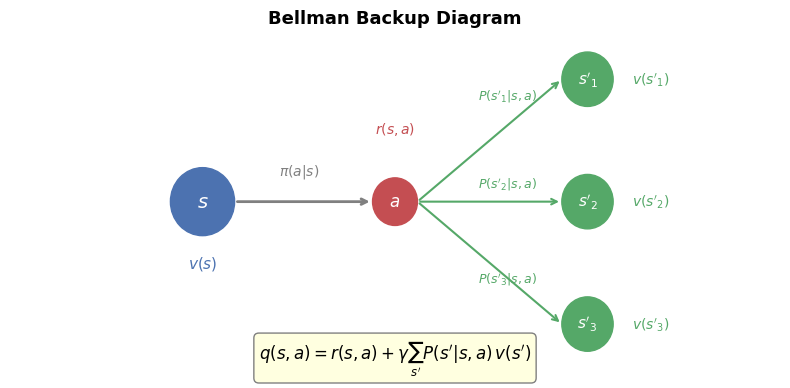
# Illustrate the Bellman backup: how v(s) depends on v(s') for successor states

fig, ax = plt.subplots(1, 1, figsize=(8, 4))
ax.set_xlim(-1, 11)
ax.set_ylim(-0.5, 4.5)
ax.axis('off')

# Central state
center_x, center_y = 2, 2
circle_s = plt.Circle((center_x, center_y), 0.5, color='#4C72B0', zorder=5)
ax.add_patch(circle_s)
ax.text(center_x, center_y, '$s$', ha='center', va='center', fontsize=14,
        color='white', fontweight='bold', zorder=6)
ax.text(center_x, center_y - 0.9, '$v(s)$', ha='center', va='center', fontsize=11, color='#4C72B0')

# Action node
action_x, action_y = 5, 2
circle_a = plt.Circle((action_x, action_y), 0.35, color='#C44E52', zorder=5)
ax.add_patch(circle_a)
ax.text(action_x, action_y, '$a$', ha='center', va='center', fontsize=12,
        color='white', fontweight='bold', zorder=6)

# Arrow from s to a
ax.annotate('', xy=(action_x - 0.35, action_y), xytext=(center_x + 0.5, center_y),
            arrowprops=dict(arrowstyle='->', lw=2, color='gray'))
ax.text(3.5, 2.4, '$\\pi(a|s)$', ha='center', fontsize=10, color='gray')

# Successor states
successors = [(8, 3.8, "$s'_1$"), (8, 2.0, "$s'_2$"), (8, 0.2, "$s'_3$")]
for sx, sy, label in successors:
    circle_sp = plt.Circle((sx, sy), 0.4, color='#55A868', zorder=5)
    ax.add_patch(circle_sp)
    ax.text(sx, sy, label, ha='center', va='center', fontsize=11,
            color='white', fontweight='bold', zorder=6)
    ax.annotate('', xy=(sx - 0.4, sy), xytext=(action_x + 0.35, action_y),
                arrowprops=dict(arrowstyle='->', lw=1.5, color='#55A868'))

# Labels
ax.text(6.3, 3.5, '$P(s\'_1|s,a)$', fontsize=9, color='#55A868')
ax.text(6.3, 2.2, '$P(s\'_2|s,a)$', fontsize=9, color='#55A868')
ax.text(6.3, 0.8, '$P(s\'_3|s,a)$', fontsize=9, color='#55A868')

# Reward label
ax.text(5, 3.0, '$r(s,a)$', ha='center', fontsize=10, color='#C44E52')

# Value labels for successors
for sx, sy, label in successors:
    vlabel = label.replace("s'", "v(s'").rstrip('$') + ')$'
    ax.text(sx + 0.7, sy, vlabel, ha='left', va='center', fontsize=10, color='#55A868')

# Equation
ax.text(5, -0.3, "$q(s,a) = r(s,a) + \\gamma \\sum_{s'} P(s'|s,a) \\, v(s')$",
        ha='center', fontsize=12, style='italic',
        bbox=dict(boxstyle='round,pad=0.3', facecolor='lightyellow', edgecolor='gray'))

ax.set_title('Bellman Backup Diagram', fontsize=13, fontweight='bold')
plt.tight_layout()
plt.show()

The backup diagram above shows the structure of the Bellman equation. The value of state \(s\) depends on the action \(a\) selected by the policy (with probability \(\pi(a \mid s)\)), the immediate reward \(r(s, a)\), and the values of the successor states \(s'\) weighted by the transition probabilities \(P(s' \mid s, a)\) and discounted by \(\gamma\).

---

6. Solving RL: Tabular Methods

Tabular RL algorithms maintain explicit tables for \(v(s)\), \(q(s, a)\), or \(\pi(s)\), with one entry per state or state-action pair. These methods are applicable when the state and action spaces are finite and small enough to enumerate. While they do not scale to large problems, they are foundational — nearly all modern RL algorithms are generalizations of tabular ideas.

Tabular methods are divided into model-based methods (which assume knowledge of the MDP dynamics) and model-free methods (which learn from experience alone).

6.1 Model-Based Methods: Dynamic Programming

Dynamic programming (DP) algorithms assume perfect knowledge of the transition probabilities \(P(s' \mid s, a)\) and the reward function \(r(s, a)\). They use the Bellman equations directly to compute value functions.

The algorithm alternates between two steps:

ImportantPolicy Evaluation and Improvement

Policy evaluation — compute \(v^\pi\) by sweeping through all states:

\[ v(s_t) \leftarrow \sum_{a_t} \pi(a_t \mid s_t) \left( r(s_t, a_t) + \gamma \sum_{s_{t+1}} P(s_{t+1} \mid s_t, a_t) \, v(s_{t+1}) \right). \]

Policy improvement — update the policy greedily:

\[ \pi(a_t \mid s_t) \leftarrow \arg\max_{a_t} \left[ r(s_t, a_t) + \gamma \sum_{s_{t+1}} P(s_{t+1} \mid s_t, a_t) \, v(s_{t+1}) \right]. \]

Each update makes \(v(s_t)\) consistent with the values of successor states — this is called bootstrapping. The policy improvement theorem guarantees this process converges to optimality.

There are two main variants:

• Policy iteration: iterate policy evaluation to convergence, then do one policy improvement step, and repeat.
• Value iteration: do only one sweep of policy evaluation before each policy improvement, combining both steps.

# Demonstrate value iteration on a simple 4x4 grid world
# Reward: +1 at state (3,3), -1 at state (2,3) (hole), 0 elsewhere
# Actions: up(0), right(1), down(2), left(3)
# Deterministic transitions (no slipping for clarity)

rows, cols = 4, 4
gamma = 0.9
n_actions = 4

# Reward grid
reward_grid = np.zeros((rows, cols))
reward_grid[3, 3] = 1.0   # fish (goal)
reward_grid[2, 3] = -1.0  # hole

# Terminal states
terminal = {(3, 3), (2, 3)}

def step(r, c, action):
    """Return next (row, col) given action. Stays in place if hitting a wall."""
    dr = [-1, 0, 1, 0]  # up, right, down, left
    dc = [0, 1, 0, -1]
    nr, nc = r + dr[action], c + dc[action]
    if 0 <= nr < rows and 0 <= nc < cols:
        return nr, nc
    return r, c

# Value iteration
V = np.zeros((rows, cols))
history = [V.copy()]
n_iterations = 20

for it in range(n_iterations):
    V_new = np.zeros((rows, cols))
    for r in range(rows):
        for c in range(cols):
            if (r, c) in terminal:
                V_new[r, c] = reward_grid[r, c]
                continue
            values = []
            for a in range(n_actions):
                nr, nc = step(r, c, a)
                values.append(reward_grid[r, c] + gamma * V[nr, nc])
            V_new[r, c] = max(values)
    V = V_new
    history.append(V.copy())

# Plot convergence: iterations 0, 2, 5, 19
show_iters = [0, 2, 5, 19]
fig, axes = plt.subplots(1, 4, figsize=(14, 3.5))

for idx, it in enumerate(show_iters):
    ax = axes[idx]
    im = ax.imshow(history[it], cmap='RdYlGn', vmin=-1, vmax=1)
    for r in range(rows):
        for c in range(cols):
            ax.text(c, r, f'{history[it][r, c]:.2f}', ha='center', va='center',
                    fontsize=10, fontweight='bold')
    ax.set_title(f'Iteration {it}', fontsize=11, fontweight='bold')
    ax.set_xticks([])
    ax.set_yticks([])

fig.suptitle('Value Iteration: Convergence of $v(s)$', fontsize=13, fontweight='bold', y=1.02)
plt.tight_layout()
plt.show()

# Show the optimal policy derived from the converged value function

arrows = ['\u2191', '\u2192', '\u2193', '\u2190']  # up, right, down, left

fig, axes = plt.subplots(1, 2, figsize=(9, 4))

# Left: converged values
ax = axes[0]
im = ax.imshow(V, cmap='RdYlGn', vmin=-1, vmax=1)
for r in range(rows):
    for c in range(cols):
        ax.text(c, r, f'{V[r, c]:.2f}', ha='center', va='center',
                fontsize=12, fontweight='bold')
ax.set_title('Converged Values $v^*(s)$', fontsize=12, fontweight='bold')
ax.set_xticks([])
ax.set_yticks([])

# Right: derived optimal policy
ax = axes[1]
ax.set_xlim(-0.5, 3.5)
ax.set_ylim(-0.5, 3.5)
ax.set_aspect('equal')
ax.invert_yaxis()

for r in range(rows):
    for c in range(cols):
        if (r, c) == (3, 3):
            color = '#abebc6'
            label = 'G'
        elif (r, c) == (2, 3):
            color = '#f5b7b1'
            label = 'X'
        else:
            color = '#d6eaf8'
            # Find best action
            best_a = 0
            best_val = -float('inf')
            for a in range(n_actions):
                nr, nc = step(r, c, a)
                val = reward_grid[r, c] + gamma * V[nr, nc]
                if val > best_val:
                    best_val = val
                    best_a = a
            label = arrows[best_a]
        rect = plt.Rectangle((c - 0.5, r - 0.5), 1, 1, fill=True,
                              facecolor=color, edgecolor='#2c3e50', linewidth=1.5)
        ax.add_patch(rect)
        ax.text(c, r, label, ha='center', va='center', fontsize=16, fontweight='bold')

ax.set_title('Optimal Policy $\\pi^*(s)$', fontsize=12, fontweight='bold')
ax.set_xticks([])
ax.set_yticks([])

plt.tight_layout()
plt.show()

The value iteration example above uses a 4x4 grid with a goal (G, reward \(+1\)) at the bottom-right and a hole (X, reward \(-1\)) just above it. At iteration 0, all values are zero. After a few iterations, the values begin to reflect the proximity to rewards and penalties. By iteration 19, the values have converged to \(v^*(s)\), and the derived optimal policy steers the agent toward the goal while avoiding the hole.

6.2 Model-Free Methods: Monte Carlo

Unlike dynamic programming, Monte Carlo (MC) methods do not assume knowledge of the MDP’s transition probabilities or reward structure. Instead, they learn from experience by repeatedly sampling complete episodes and observing the rewards.

NoteMonte Carlo Method

1. Generate episodes using the current policy \(\pi\).
2. Estimate action values \(q(s, a)\) as the average of the empirical returns observed each time \((s, a)\) is visited.
3. Improve the policy greedily:

\[ \pi(a \mid s) \leftarrow \arg\max_a \, q(s, a). \]

MC methods require complete episodes before learning. An \(\varepsilon\)-greedy policy (random action with probability \(\varepsilon\), greedy with \(1 - \varepsilon\)) is used to ensure exploration.

# Monte Carlo estimation example on the grid world
# Simulate episodes and estimate Q-values

np.random.seed(0)

Q = np.zeros((rows, cols, n_actions))
returns_count = np.zeros((rows, cols, n_actions))
returns_sum = np.zeros((rows, cols, n_actions))
epsilon = 0.2
n_episodes = 2000
max_steps = 50

avg_returns = []

for ep in range(n_episodes):
    # Generate an episode using epsilon-greedy policy
    episode = []
    r, c = np.random.randint(0, rows), np.random.randint(0, cols)
    while (r, c) in terminal:
        r, c = np.random.randint(0, rows), np.random.randint(0, cols)

    for t in range(max_steps):
        if np.random.random() < epsilon:
            action = np.random.randint(n_actions)
        else:
            action = np.argmax(Q[r, c])
        nr, nc = step(r, c, action)
        reward = reward_grid[r, c]
        episode.append((r, c, action, reward))
        r, c = nr, nc
        if (r, c) in terminal:
            episode.append((r, c, 0, reward_grid[r, c]))
            break

    # Compute returns and update Q-values (first-visit MC)
    G = 0
    visited = set()
    for t in reversed(range(len(episode))):
        sr, sc, sa, sr_reward = episode[t]
        G = gamma * G + sr_reward
        if (sr, sc, sa) not in visited:
            visited.add((sr, sc, sa))
            returns_sum[sr, sc, sa] += G
            returns_count[sr, sc, sa] += 1
            Q[sr, sc, sa] = returns_sum[sr, sc, sa] / returns_count[sr, sc, sa]

    avg_returns.append(G)

# Plot learning curve
window = 50
smoothed = np.convolve(avg_returns, np.ones(window)/window, mode='valid')

fig, axes = plt.subplots(1, 2, figsize=(11, 4))

ax = axes[0]
ax.plot(smoothed, color='#4C72B0', linewidth=1.5)
ax.set_xlabel('Episode', fontsize=11)
ax.set_ylabel('Average Return (smoothed)', fontsize=11)
ax.set_title('Monte Carlo Learning Curve', fontsize=12, fontweight='bold')
ax.grid(True, alpha=0.3)

# Show the derived policy
ax = axes[1]
ax.set_xlim(-0.5, 3.5)
ax.set_ylim(-0.5, 3.5)
ax.set_aspect('equal')
ax.invert_yaxis()
for r in range(rows):
    for c in range(cols):
        if (r, c) == (3, 3):
            color, label = '#abebc6', 'G'
        elif (r, c) == (2, 3):
            color, label = '#f5b7b1', 'X'
        else:
            color = '#d6eaf8'
            best_a = np.argmax(Q[r, c])
            label = arrows[best_a]
        rect = plt.Rectangle((c - 0.5, r - 0.5), 1, 1, fill=True,
                              facecolor=color, edgecolor='#2c3e50', linewidth=1.5)
        ax.add_patch(rect)
        ax.text(c, r, label, ha='center', va='center', fontsize=16, fontweight='bold')
ax.set_title('Policy from Monte Carlo', fontsize=12, fontweight='bold')
ax.set_xticks([])
ax.set_yticks([])

plt.tight_layout()
plt.show()

The left panel shows the learning curve: the average return per episode increases as the agent accumulates experience. The right panel shows the policy derived from Monte Carlo estimation after 2000 episodes. Note that unlike dynamic programming, Monte Carlo needed no knowledge of transition probabilities — it learned entirely from sampled trajectories.

6.3 Temporal Difference (TD) Methods

Temporal difference methods combine the best of dynamic programming and Monte Carlo. Like Monte Carlo, they learn from experience without knowing the model. Like dynamic programming, they update estimates based on other estimates (bootstrapping) rather than waiting for a complete episode.

ImportantTD Error

The core idea is the TD error:

\[ \delta_t = r_{t+1} + \gamma \cdot V(s_{t+1}) - V(s_t), \]

which measures the discrepancy between the current estimate \(V(s_t)\) and the improved estimate \(r_{t+1} + \gamma V(s_{t+1})\) obtained after taking one step.

The TD error is the difference between two successive estimates. When this error is zero, the Bellman equation is satisfied and the value function is consistent.

SARSA (On-Policy)

ImportantSARSA Update

SARSA (State-Action-Reward-State-Action) updates the action value using the action actually taken:

\[ q(s_t, a_t) \leftarrow q(s_t, a_t) + \alpha \Big( r(s_t, a_t) + \gamma \cdot q(s_{t+1}, a_{t+1}) - q(s_t, a_t) \Big). \]

SARSA is on-policy: it learns values for the policy it is currently following, including exploration. This makes it more conservative in risky environments.

Q-Learning (Off-Policy)

ImportantQ-Learning Update

Q-learning updates the action value using the maximum action value at the next state:

\[ q(s_t, a_t) \leftarrow q(s_t, a_t) + \alpha \Big( r(s_t, a_t) + \gamma \cdot \max_a q(s_{t+1}, a) - q(s_t, a_t) \Big). \]

Q-learning is off-policy: it learns the optimal values \(q^*\) even while following an exploratory policy. The separation of behavior policy (exploration) from target policy (greedy) is the hallmark of off-policy methods.

# Compare SARSA and Q-learning on the grid world

def run_td(method='q-learning', n_episodes=1500, alpha=0.1, epsilon=0.1, gamma=0.9, seed=42):
    np.random.seed(seed)
    Q = np.zeros((rows, cols, n_actions))
    episode_returns = []

    for ep in range(n_episodes):
        r, c = 0, 0  # start at top-left
        # epsilon-greedy action selection
        if np.random.random() < epsilon:
            action = np.random.randint(n_actions)
        else:
            action = np.argmax(Q[r, c])

        total_return = 0
        for t in range(100):
            nr, nc = step(r, c, action)
            reward = reward_grid[r, c]
            total_return += (gamma ** t) * reward

            if (nr, nc) in terminal:
                total_return += (gamma ** (t+1)) * reward_grid[nr, nc]
                if method == 'q-learning':
                    Q[r, c, action] += alpha * (reward + gamma * reward_grid[nr, nc] - Q[r, c, action])
                else:  # SARSA
                    Q[r, c, action] += alpha * (reward + gamma * reward_grid[nr, nc] - Q[r, c, action])
                break

            # Next action
            if np.random.random() < epsilon:
                next_action = np.random.randint(n_actions)
            else:
                next_action = np.argmax(Q[nr, nc])

            if method == 'q-learning':
                td_target = reward + gamma * np.max(Q[nr, nc])
            else:  # SARSA
                td_target = reward + gamma * Q[nr, nc, next_action]

            Q[r, c, action] += alpha * (td_target - Q[r, c, action])
            r, c = nr, nc
            action = next_action

        episode_returns.append(total_return)

    return Q, episode_returns

Q_qlearn, returns_qlearn = run_td('q-learning')
Q_sarsa, returns_sarsa = run_td('sarsa')

# Smooth and plot
window = 50
smooth_q = np.convolve(returns_qlearn, np.ones(window)/window, mode='valid')
smooth_s = np.convolve(returns_sarsa, np.ones(window)/window, mode='valid')

fig, axes = plt.subplots(1, 3, figsize=(14, 4))

# Learning curves
ax = axes[0]
ax.plot(smooth_q, label='Q-Learning', color='#C44E52', linewidth=1.5)
ax.plot(smooth_s, label='SARSA', color='#4C72B0', linewidth=1.5)
ax.set_xlabel('Episode', fontsize=11)
ax.set_ylabel('Return (smoothed)', fontsize=11)
ax.set_title('TD Learning Curves', fontsize=12, fontweight='bold')
ax.legend()
ax.grid(True, alpha=0.3)

# Q-learning policy
for idx, (Q_val, title) in enumerate([(Q_qlearn, 'Q-Learning Policy'), (Q_sarsa, 'SARSA Policy')]):
    ax = axes[idx + 1]
    ax.set_xlim(-0.5, 3.5)
    ax.set_ylim(-0.5, 3.5)
    ax.set_aspect('equal')
    ax.invert_yaxis()
    for r in range(rows):
        for c in range(cols):
            if (r, c) == (3, 3):
                color, label = '#abebc6', 'G'
            elif (r, c) == (2, 3):
                color, label = '#f5b7b1', 'X'
            else:
                color = '#d6eaf8'
                best_a = np.argmax(Q_val[r, c])
                label = arrows[best_a]
            rect = plt.Rectangle((c - 0.5, r - 0.5), 1, 1, fill=True,
                                  facecolor=color, edgecolor='#2c3e50', linewidth=1.5)
            ax.add_patch(rect)
            ax.text(c, r, label, ha='center', va='center', fontsize=16, fontweight='bold')
    ax.set_title(title, fontsize=12, fontweight='bold')
    ax.set_xticks([])
    ax.set_yticks([])

plt.tight_layout()
plt.show()

The figure compares Q-learning and SARSA on the same grid world. Both methods learn step-by-step without waiting for complete episodes. Q-learning (off-policy) learns the optimal policy directly, while SARSA (on-policy) learns the value of the policy it is actually following (including exploration). In practice, SARSA tends to be more conservative because it accounts for the randomness introduced by the \(\varepsilon\)-greedy exploration policy.

NoteComparison of Tabular Methods

	Dynamic Programming	Monte Carlo	Temporal Difference
Requires model?	Yes (\(P\), \(r\) known)	No	No
Updates from	Bellman equations	Complete episodes	Single steps (bootstrap)
Bias/Variance	No sampling bias	High variance	Low variance, some bias
Works online?	No (full sweep)	No (needs full episode)	Yes
Key algorithms	Policy/Value iteration	First-visit MC	SARSA, Q-learning

---

7. Limitations of Tabular RL

Tabular methods provide a clean and complete framework for solving small MDPs, but they have fundamental scalability limitations:

• Discrete states and actions required: Tabular methods maintain one entry per state or state-action pair. They cannot directly handle continuous state spaces (e.g., joint angles of a robot) or continuous action spaces (e.g., torques).

• Small state-action spaces only: Even for constrained environments, state spaces can be enormous. A chessboard has more than \(10^{40}\) possible legal states. A video game frame at \(84 \times 84\) grayscale resolution has \(256^{84 \times 84}\) possible observations. Storing a table entry for each is clearly infeasible.

• No generalization: Tabular methods treat each state independently. Learning that one state is good tells us nothing about similar states nearby. This means the agent must visit every state many times, which is impractical in large environments.

These limitations motivate the use of function approximation, where value functions or policies are represented by parameterized models (e.g., neural networks) that can generalize across states. This leads to deep reinforcement learning, where deep networks replace the explicit tables — a topic we will explore in subsequent lessons.

# Visualize the explosion of state space size

problems = ['4x4 Grid\n(16 states)', 'Chess\n(~$10^{40}$ states)', 'Go\n(~$10^{170}$ states)',
            'Atari Frame\n($256^{7056}$ states)', 'Robotics\n(continuous)']
log_sizes = [np.log10(16), 40, 170, 7056 * np.log10(256), None]  # last is infinite
colors = ['#55A868', '#4C72B0', '#8172B2', '#C44E52', '#CCB974']

fig, ax = plt.subplots(1, 1, figsize=(9, 4))

# Only plot finite ones
bar_vals = log_sizes[:4]
bar_labels = problems[:4]
bar_colors = colors[:4]

bars = ax.bar(range(len(bar_vals)), bar_vals, color=bar_colors, edgecolor='black', linewidth=1)

# Add the continuous one as a special marker
ax.bar(4, max(bar_vals) * 1.15, color=colors[4], edgecolor='black', linewidth=1, hatch='//')
ax.text(4, max(bar_vals) * 1.15 + 200, '$\\infty$', ha='center', fontsize=14, fontweight='bold')

ax.set_xticks(range(5))
ax.set_xticklabels(problems, fontsize=9)
ax.set_ylabel('$\\log_{10}$(State Space Size)', fontsize=11)
ax.set_title('State Space Sizes: Why Tabular Methods Do Not Scale', fontsize=12, fontweight='bold')

# Add a horizontal line for "tabular feasible" region
ax.axhline(y=6, color='red', linestyle='--', alpha=0.7)
ax.text(0.5, 6 + 200, 'Tabular feasible (~$10^6$ states)', fontsize=9, color='red')

ax.grid(True, alpha=0.2, axis='y')
plt.tight_layout()
plt.show()

The chart illustrates why tabular methods cannot scale beyond toy problems. Even chess has roughly \(10^{40}\) states — far beyond what any table can store. For image-based domains like Atari or continuous robotics tasks, function approximation via neural networks is essential.

---

8. Summary

This lesson covered the foundations of reinforcement learning, building from the simplest models to practical solution methods:

• RL setup: An agent interacts with an environment in a loop — observing states, taking actions, receiving rewards — with the goal of maximizing cumulative reward.

• Markov processes to MDPs: We built up through Markov processes (states + transitions), Markov reward processes (adding rewards and discounting), and finally Markov decision processes (adding actions and policies).

• Policies and trajectories: A policy \(\pi(a \mid s)\) defines the agent’s behavior. It can be deterministic or stochastic. Trajectories are sequences of states, actions, and rewards.

• Objective: The agent seeks to maximize the expected return \(G_t = \sum_{k=0}^{\infty} \gamma^k r_{t+k+1}\).

• Value functions: The state value \(v^\pi(s)\) and action value \(q^\pi(s, a)\) quantify the long-term reward under a policy. The optimal policy chooses actions that maximize \(q^*(s, a)\).

• Bellman equations: The recursive relationship \(q(s, a) = r(s, a) + \gamma \sum_{s'} P(s' \mid s, a) v(s')\) is the foundation of all RL algorithms.

• Solution methods:

  • Dynamic programming (model-based): Uses the Bellman equations with known dynamics for iterative policy evaluation and improvement.
  • Monte Carlo (sampling-based): Learns from complete episodes without a model.
  • Temporal difference (hybrid): Combines sampling and bootstrapping for online, step-by-step learning. SARSA is on-policy; Q-learning is off-policy.

• Limitation: Tabular methods require discrete, small state-action spaces. For real-world problems with large or continuous state spaces, function approximation (deep RL) is necessary.

References

1. Simon J.D. Prince, “Understanding Deep Learning”, Chapter 19: Reinforcement Learning,