Deep Q-Networks

reinforcement learning

deep learning

DQN

From temporal difference methods (SARSA, Q-learning) to deep Q-networks and double DQN — scaling RL to high-dimensional state spaces.

Published

April 1, 2026

Abstract

This lesson covers neural network based reinforcement learning, building from tabular temporal difference (TD) methods to deep Q-networks (DQN). We begin with the SARSA and Q-learning algorithms that update action values from single transitions. We then move to fitted Q-learning, where a neural network approximates the Q-function over continuous, high-dimensional state spaces. The core of the lesson describes Deep Q-Networks — the architecture that learned to play Atari games from raw pixels — along with the training tricks that make it work: fixed target networks, experience replay, and reward clipping. Finally, we introduce double Q-learning and double DQN, which correct the systematic overestimation bias inherent in the max operator.

CREATED AT: 2026-04-01

1. Q-Learning Using Temporal Difference Methods

In the previous lesson we introduced the Bellman equations and three families of tabular RL methods: dynamic programming, Monte Carlo, and temporal difference (TD). Dynamic programming requires a full model of the environment; Monte Carlo methods require complete episodes. Temporal difference methods combine the best of both worlds: they learn directly from experience (like Monte Carlo) and update estimates based on other estimates without waiting for the episode to end (like dynamic programming).

In this section we look at two foundational TD algorithms for estimating the action-value function \(q[s, a]\): SARSA and Q-learning.

1.1 SARSA

SARSA (State-Action-Reward-State-Action) is an on-policy TD algorithm. Its name comes from the quintuple \((s_t, a_t, r_{t+1}, s_{t+1}, a_{t+1})\) used in each update.

SARSA Update Rule

\[ q[s_t, a_t] \leftarrow q[s_t, a_t] + \alpha\Big(r[s_t, a_t] + \gamma \cdot q[s_{t+1}, a_{t+1}] - q[s_t, a_t]\Big) \]

where \(\alpha \in \mathbb{R}^+\) is the learning rate. The bracketed quantity

\[ \delta_t = r[s_t, a_t] + \gamma \cdot q[s_{t+1}, a_{t+1}] - q[s_t, a_t] \]

is called the TD error. It measures the discrepancy between the current estimate \(q[s_t, a_t]\) and the bootstrapped target \(r[s_t, a_t] + \gamma \cdot q[s_{t+1}, a_{t+1}]\).

The TD error drives learning: when the agent receives a better-than-expected outcome (\(\delta_t > 0\)), the action value is revised upward; when the outcome is worse (\(\delta_t < 0\)), it is revised downward.

SARSA Algorithm (Pseudocode)

Initialize q[s, a] arbitrarily for all s, a
for each episode:
    Initialize state s
    Choose action a from s using policy derived from q
        (e.g., epsilon-greedy)
    for each step of the episode:
        Take action a, observe reward r and next state s'
        Choose action a' from s' using policy derived from q
            (e.g., epsilon-greedy)
        q[s, a] <- q[s, a] + alpha * (r + gamma * q[s', a'] - q[s, a])
        s <- s'
        a <- a'
    until s is terminal

SARSA is an on-policy algorithm: the same policy that the agent follows to explore the environment is the one whose value function is being estimated. In practice, this policy is typically \(\epsilon\)-greedy — the agent takes a random action with probability \(\epsilon\) and the greedy action with probability \(1 - \epsilon\). Because the update uses \(a_{t+1}\), which is chosen by this same policy, the estimated values reflect the actual behavior of the agent, including its exploratory moves.

It can be shown that the SARSA updates are contraction mappings, guaranteeing convergence to the optimal action-value function (assuming every state-action pair is visited infinitely often and the learning rate schedule satisfies the Robbins-Monro conditions).

1.2 Q-Learning

Q-learning modifies the SARSA update by replacing \(q[s_{t+1}, a_{t+1}]\) with \(\max_a q[s_{t+1}, a]\). This single change has a profound consequence: the update no longer depends on the action the agent actually takes next.

Q-Learning Update Rule

\[ q[s_t, a_t] \leftarrow q[s_t, a_t] + \alpha\Big(r[s_t, a_t] + \gamma \cdot \max_a\big[q[s_{t+1}, a]\big] - q[s_t, a_t]\Big) \]

The key difference from SARSA: the target uses the maximum action value at \(s_{t+1}\), regardless of which action the agent actually takes.

Q-Learning Algorithm (Pseudocode)

Initialize q[s, a] arbitrarily for all s, a
for each episode:
    Initialize state s
    for each step of the episode:
        Choose action a from s using behaviour policy pi'
            (e.g., epsilon-greedy w.r.t. q)
        Take action a, observe reward r and next state s'
        q[s, a] <- q[s, a] + alpha * (r + gamma * max_a'(q[s', a']) - q[s, a])
        s <- s'
    until s is terminal

Q-learning is an off-policy algorithm. The agent follows a behaviour policy \(\pi'\) (e.g., \(\epsilon\)-greedy) to explore the environment, but the update targets the greedy policy — the one that always picks the action with the highest Q-value. This decoupling is powerful: the agent can explore freely using \(\pi'\) while still learning the optimal Q-function.

Like SARSA, the Q-learning updates are contraction mappings, and the algorithm converges to the optimal action-value function \(q^*[s, a]\) under the same visiting and learning-rate conditions.

2. Deep Q-Networks

The tabular methods of Section 1 maintain a lookup table with one entry for every state-action pair. This is only practical when the state space is small. In many real-world problems, the state is a dense vector \(\mathbf{s}_t \in \mathbb{R}^d\) — for example, pixel values on a screen, joint angles of a robot, or readings from a sensor array. Even for discrete problems like chess, the number of possible board configurations exceeds \(10^{40}\), making a table infeasible.

The idea behind fitted Q-learning and deep Q-networks is to replace the table with a parameterized function approximator — in particular, a neural network — that maps state vectors (and actions) to Q-values:

\[ q[\mathbf{s}, a \mid \boldsymbol{\phi}] \in \mathbb{R} \]

With a finite action set \(\mathcal{A}\), a single forward pass through the network can output a vector \(q[\mathbf{s} \mid \boldsymbol{\phi}] \in \mathbb{R}^{|\mathcal{A}|}\), giving the value for every action simultaneously.

2.1 Fitted Q-Learning

Fitted Q-learning replaces the discrete table \(q[s, a]\) with a differentiable model \(q[\mathbf{s}, a, \boldsymbol{\phi}]\) parameterized by weights \(\boldsymbol{\phi}\). The TD error now becomes a continuous function of the parameters.

Least-Squares Loss on the TD Error

\[ L[\boldsymbol{\phi}] = \left(r[\mathbf{s}_t, a_t] + \gamma \cdot \max_a\Big[q[\mathbf{s}_{t+1}, a, \boldsymbol{\phi}]\Big] - q[\mathbf{s}_t, a_t, \boldsymbol{\phi}]\right)^2 \]

This loss measures the squared TD error: how far the current Q-prediction is from the bootstrapped target.

The target \(r[\mathbf{s}_t, a_t] + \gamma \cdot \max_a[q[\mathbf{s}_{t+1}, a, \boldsymbol{\phi}]]\) itself depends on \(\boldsymbol{\phi}\). This creates a moving target problem — the goal shifts every time we update the weights.

Taking the gradient of \(L\) with respect to \(\boldsymbol{\phi}\) and applying gradient descent yields the update rule:

Fitted Q-Learning Update Rule

\[ \boldsymbol{\phi} \leftarrow \boldsymbol{\phi} + \alpha\left(r[\mathbf{s}_t, a_t] + \gamma \cdot \max_a\Big[q[\mathbf{s}_{t+1}, a, \boldsymbol{\phi}]\Big] - q[\mathbf{s}_t, a_t, \boldsymbol{\phi}]\right)\frac{\partial\, q[\mathbf{s}_t, a_t, \boldsymbol{\phi}]}{\partial \boldsymbol{\phi}} \]

This is obtained by computing \(\partial L / \partial \boldsymbol{\phi}\), treating the target as a constant (a common semi-gradient trick).

No Convergence Guarantee

Unlike tabular Q-learning, fitted Q-learning does not guarantee convergence. The problem is that a change to \(\boldsymbol{\phi}\) modifies both the prediction \(q[\mathbf{s}_t, a_t, \boldsymbol{\phi}]\) and the target \(r + \gamma \max_a q[\mathbf{s}_{t+1}, a, \boldsymbol{\phi}]\) simultaneously. This can lead to oscillation or divergence.

2.2 Deep Q-Network (DQN) for Playing Games

The Deep Q-Network (DQN), introduced by Mnih et al. at DeepMind (2013, 2015), was the first architecture to successfully combine deep learning with reinforcement learning at scale. It learned to play 49 Atari 2600 games directly from raw screen pixels, achieving human-level performance in many of them.

The state representation is a stack of 4 consecutive grayscale frames, each resized to \(84 \times 84\) pixels, giving \(\mathbf{s}_t \in \mathbb{R}^{4 \times 84 \times 84}\). The network outputs one Q-value for each of the 18 possible Atari actions.

Show code

import matplotlib.pyplot as plt
import matplotlib.patches as mpatches
import numpy as np

fig, ax = plt.subplots(1, 1, figsize=(12, 5))
ax.set_xlim(0, 16)
ax.set_ylim(0, 7)
ax.axis('off')
ax.set_title('Deep Q-Network (DQN) Architecture', fontsize=14, fontweight='bold', pad=15)

# --- Input: 4 stacked frames ---
for i in range(4):
    rect = mpatches.FancyBboxPatch(
        (0.3 + i * 0.15, 3 - i * 0.15), 1.4, 1.8,
        boxstyle='round,pad=0.05', facecolor=plt.cm.Greys(0.3 + i * 0.15),
        edgecolor='black', linewidth=1, alpha=0.85
    )
    ax.add_patch(rect)
ax.text(1.05, 2, 'Input\n$4 \\times 84 \\times 84$\ngrayscale frames', ha='center',
        fontsize=8, va='top')

# --- Conv layers ---
conv_specs = [
    ('Conv1\n$8{\\times}8$\nstride 4\n16 filters', 3.2, '#4C72B0', 1.0, 1.6),
    ('Conv2\n$4{\\times}4$\nstride 2\n32 filters', 5.4, '#4C72B0', 0.85, 1.35),
    ('Conv3\n$3{\\times}3$\nstride 1\n32 filters', 7.4, '#4C72B0', 0.7, 1.1),
]

layer_centers = [1.05]  # input center x
for label, x, color, w, h in conv_specs:
    rect = mpatches.FancyBboxPatch(
        (x, 3.5 - h / 2), w, h,
        boxstyle='round,pad=0.08', facecolor=color, edgecolor='black',
        linewidth=1.5, alpha=0.9
    )
    ax.add_patch(rect)
    ax.text(x + w / 2, 3.5, label, ha='center', va='center',
            fontsize=7, color='white', fontweight='bold')
    layer_centers.append(x + w / 2)

# --- FC layers ---
fc_specs = [
    ('FC1\n256 units', 9.5, '#55A868', 0.9, 1.0),
    ('FC2\n18 units', 11.5, '#55A868', 0.9, 1.0),
]
for label, x, color, w, h in fc_specs:
    rect = mpatches.FancyBboxPatch(
        (x, 3.5 - h / 2), w, h,
        boxstyle='round,pad=0.08', facecolor=color, edgecolor='black',
        linewidth=1.5, alpha=0.9
    )
    ax.add_patch(rect)
    ax.text(x + w / 2, 3.5, label, ha='center', va='center',
            fontsize=8, color='white', fontweight='bold')
    layer_centers.append(x + w / 2)

# --- Output: Q-values ---
out_x = 13.3
n_actions = 6  # Show 6 representative outputs
labels_out = ['$q(\\mathbf{s},a_1)$', '$q(\\mathbf{s},a_2)$', '$q(\\mathbf{s},a_3)$',
              '...', '$q(\\mathbf{s},a_{17})$', '$q(\\mathbf{s},a_{18})$']
y_positions = np.linspace(1.5, 5.5, n_actions)
for y, lab in zip(y_positions, labels_out):
    rect = mpatches.FancyBboxPatch(
        (out_x, y - 0.2), 1.8, 0.4,
        boxstyle='round,pad=0.05', facecolor='#C44E52', edgecolor='black',
        linewidth=1, alpha=0.9
    )
    ax.add_patch(rect)
    ax.text(out_x + 0.9, y, lab, ha='center', va='center',
            fontsize=8, color='white', fontweight='bold')
layer_centers.append(out_x + 0.9)

ax.text(out_x + 0.9, 0.8, 'Output\nQ-values\n(18 actions)', ha='center',
        fontsize=8, va='top')

# --- Arrows between layers ---
arrow_xs = [
    (1.05 + 0.75, 3.2),            # input -> conv1
    (3.2 + 1.0, 5.4),              # conv1 -> conv2
    (5.4 + 0.85, 7.4),             # conv2 -> conv3
    (7.4 + 0.7, 9.5),              # conv3 -> fc1
    (9.5 + 0.9, 11.5),             # fc1 -> fc2
    (11.5 + 0.9, out_x),           # fc2 -> output
]
for x_start, x_end in arrow_xs:
    ax.annotate('', xy=(x_end, 3.5), xytext=(x_start, 3.5),
                arrowprops=dict(arrowstyle='->', lw=1.5, color='gray'))

plt.tight_layout()
plt.show()

The DQN architecture consists of:

Input: 4 consecutive \(84 \times 84\) grayscale frames (to capture motion/velocity information)
Conv layer 1: 16 filters of size \(8 \times 8\) with stride 4
Conv layer 2: 32 filters of size \(4 \times 4\) with stride 2
Conv layer 3: 32 filters of size \(3 \times 3\) with stride 1
Fully connected layer 1: 256 hidden units
Output layer: one Q-value per action (18 actions for Atari)

However, like fitted Q-learning, training this network with standard stochastic gradient descent on the TD loss may not converge, because the target depends on the parameters being optimized.

2.3 Training the Q-Network

The DQN paper introduced several crucial modifications to make training stable. These tricks address the moving-target and correlated-sample problems that plague naive fitted Q-learning.

Fixed Target Network

The central idea is to maintain a separate copy of the network parameters, denoted \(\boldsymbol{\phi}^-\), which is held fixed for many update steps. The target Q-value is computed using \(\boldsymbol{\phi}^-\), while the gradient update is applied to \(\boldsymbol{\phi}\):

DQN Update Rule with Fixed Target

\[ \boldsymbol{\phi} \leftarrow \boldsymbol{\phi} + \alpha\left(r[\mathbf{s}_t, a_t] + \gamma \cdot \max_a\Big[q[\mathbf{s}_{t+1}, a, \boldsymbol{\phi}^-]\Big] - q[\mathbf{s}_t, a_t, \boldsymbol{\phi}]\right)\frac{\partial\, q[\mathbf{s}_t, a_t, \boldsymbol{\phi}]}{\partial \boldsymbol{\phi}} \]

Periodically (e.g., every \(C\) steps), the target parameters are synchronized: \(\boldsymbol{\phi}^- \leftarrow \boldsymbol{\phi}\).

By freezing \(\boldsymbol{\phi}^-\), the target no longer shifts with every gradient step. The network effectively chases a stationary target for \(C\) steps at a time, reducing oscillation.

Experience Replay

Consecutive frames in a game are highly correlated. Training on them sequentially violates the i.i.d. assumption of stochastic gradient descent. Experience replay stores transitions \(\langle \mathbf{s}_t, a_t, r_{t+1}, \mathbf{s}_{t+1} \rangle\) in a large buffer and samples random mini-batches for each update. This:

Breaks temporal correlations between training samples
Reuses each experience many times, improving data efficiency
Smooths out the training distribution

Reward Clipping

Atari games have vastly different score scales (some give points in the thousands, others in single digits). DQN clips all rewards to the set \(\{-1, 0, +1\}\). This ensures the same learning rate and network architecture can be used across all games without per-game tuning.

Epsilon-Greedy Exploration

The behaviour policy is \(\epsilon\)-greedy: with probability \(\epsilon\) the agent takes a random action, and with probability \(1 - \epsilon\) it takes the greedy action \(\text{argmax}_a\, q[\mathbf{s}_t, a, \boldsymbol{\phi}]\). Typically, \(\epsilon\) is annealed from a high value (e.g., 1.0) down to a small value (e.g., 0.1) over the course of training.

2.4 Double Q-Learning

Let us return to the standard Q-learning update:

\[ q[s_t, a_t] \leftarrow q[s_t, a_t] + \alpha\Big(r[s_t, a_t] + \gamma \cdot \underbrace{\max_a[q[s_{t+1}, a]]}_{\text{target selection}} - q[s_t, a_t]\Big) \]

Notice that the \(\max\) operator serves two roles simultaneously:

Target action selection: it picks the action \(a^* = \text{argmax}_a\, q[s_{t+1}, a]\)
Target value evaluation: it evaluates the value of that action using the same Q-function: \(q[s_{t+1}, a^*]\)

When the Q-values contain noise (which they always do, especially early in training), the \(\max\) operator systematically overestimates the true value. Consider two actions that both yield the same expected reward, but one has stochastic returns. The max operator will tend to select whichever estimate is noisily higher, biasing the estimate upward.

Double Q-Learning

Double Q-learning decouples action selection from value evaluation by maintaining two independent Q-functions, \(q_1\) and \(q_2\). Each Q-function selects the best action, but the other Q-function evaluates it:

\[ q_1[s_t, a_t] \leftarrow q_1[s_t, a_t] + \alpha\Big(r[s_t, a_t] + \gamma \cdot q_2\big[s_{t+1}, \text{argmax}_a[q_1[s_{t+1}, a]]\big] - q_1[s_t, a_t]\Big) \]

\[ q_2[s_t, a_t] \leftarrow q_2[s_t, a_t] + \alpha\Big(r[s_t, a_t] + \gamma \cdot q_1\big[s_{t+1}, \text{argmax}_a[q_2[s_{t+1}, a]]\big] - q_2[s_t, a_t]\Big) \]

In practice, each new experience tuple \(\langle s, a, r, s' \rangle\) is randomly assigned to update either \(q_1\) or \(q_2\).

The key insight: if \(q_1\) noisily overestimates the value of some action, \(q_2\) (being independently estimated) is unlikely to share the same bias, so the evaluated target will be closer to the true value.

2.5 Double Deep Q-Network (Double DQN)

Double Q-learning translates naturally to the neural network setting. We use the same network architecture \(q\), but with two separate sets of parameters: \(\boldsymbol{\phi}_1\) and \(\boldsymbol{\phi}_2\).

Show code

import matplotlib.pyplot as plt
import matplotlib.patches as mpatches
import numpy as np

fig, ax = plt.subplots(1, 1, figsize=(11, 6))
ax.set_xlim(0, 14)
ax.set_ylim(0, 9)
ax.axis('off')
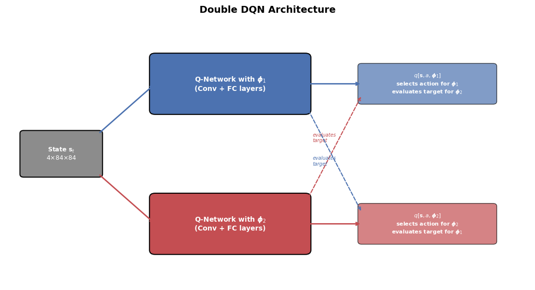
ax.set_title('Double DQN Architecture', fontsize=14, fontweight='bold', pad=15)

# --- Shared input ---
inp_box = mpatches.FancyBboxPatch(
    (0.5, 3.8), 2.0, 1.4, boxstyle='round,pad=0.1',
    facecolor='#8C8C8C', edgecolor='black', linewidth=1.5
)
ax.add_patch(inp_box)
ax.text(1.5, 4.5, 'State $\\mathbf{s}_t$\n$4{\\times}84{\\times}84$',
        ha='center', va='center', fontsize=9, color='white', fontweight='bold')

# --- Network 1 (phi_1) ---
net1_box = mpatches.FancyBboxPatch(
    (4.0, 6.0), 4.0, 1.8, boxstyle='round,pad=0.15',
    facecolor='#4C72B0', edgecolor='black', linewidth=1.5
)
ax.add_patch(net1_box)
ax.text(6.0, 6.9, 'Q-Network with $\\boldsymbol{\\phi}_1$\n(Conv + FC layers)',
        ha='center', va='center', fontsize=10, color='white', fontweight='bold')

# --- Network 2 (phi_2) ---
net2_box = mpatches.FancyBboxPatch(
    (4.0, 1.2), 4.0, 1.8, boxstyle='round,pad=0.15',
    facecolor='#C44E52', edgecolor='black', linewidth=1.5
)
ax.add_patch(net2_box)
ax.text(6.0, 2.1, 'Q-Network with $\\boldsymbol{\\phi}_2$\n(Conv + FC layers)',
        ha='center', va='center', fontsize=10, color='white', fontweight='bold')

# --- Output 1 ---
out1_box = mpatches.FancyBboxPatch(
    (9.5, 6.3), 3.5, 1.2, boxstyle='round,pad=0.1',
    facecolor='#4C72B0', edgecolor='black', linewidth=1, alpha=0.7
)
ax.add_patch(out1_box)
ax.text(11.25, 6.9, '$q[\\mathbf{s}, a, \\boldsymbol{\\phi}_1]$\nselects action for $\\boldsymbol{\\phi}_1$\nevaluates target for $\\boldsymbol{\\phi}_2$',
        ha='center', va='center', fontsize=8, color='white', fontweight='bold')

# --- Output 2 ---
out2_box = mpatches.FancyBboxPatch(
    (9.5, 1.5), 3.5, 1.2, boxstyle='round,pad=0.1',
    facecolor='#C44E52', edgecolor='black', linewidth=1, alpha=0.7
)
ax.add_patch(out2_box)
ax.text(11.25, 2.1, '$q[\\mathbf{s}, a, \\boldsymbol{\\phi}_2]$\nselects action for $\\boldsymbol{\\phi}_2$\nevaluates target for $\\boldsymbol{\\phi}_1$',
        ha='center', va='center', fontsize=8, color='white', fontweight='bold')

# --- Arrows: input -> networks ---
ax.annotate('', xy=(4.0, 6.9), xytext=(2.5, 5.2),
            arrowprops=dict(arrowstyle='->', lw=2, color='#4C72B0'))
ax.annotate('', xy=(4.0, 2.1), xytext=(2.5, 3.8),
            arrowprops=dict(arrowstyle='->', lw=2, color='#C44E52'))

# --- Arrows: networks -> outputs ---
ax.annotate('', xy=(9.5, 6.9), xytext=(8.0, 6.9),
            arrowprops=dict(arrowstyle='->', lw=2, color='#4C72B0'))
ax.annotate('', xy=(9.5, 2.1), xytext=(8.0, 2.1),
            arrowprops=dict(arrowstyle='->', lw=2, color='#C44E52'))

# --- Cross arrows (evaluation) ---
ax.annotate('', xy=(9.5, 6.5), xytext=(8.0, 2.8),
            arrowprops=dict(arrowstyle='->', lw=1.5, color='#C44E52',
                            linestyle='dashed'))
ax.text(8.2, 4.9, 'evaluates\ntarget', ha='left', fontsize=7, color='#C44E52',
        fontstyle='italic')

ax.annotate('', xy=(9.5, 2.5), xytext=(8.0, 6.2),
            arrowprops=dict(arrowstyle='->', lw=1.5, color='#4C72B0',
                            linestyle='dashed'))
ax.text(8.2, 4.1, 'evaluates\ntarget', ha='left', fontsize=7, color='#4C72B0',
        fontstyle='italic')

plt.tight_layout()
plt.show()

Double DQN Update Rules

The two parameter sets are updated as follows:

\[ \boldsymbol{\phi}_1 \leftarrow \boldsymbol{\phi}_1 + \alpha\left(r[\mathbf{s}_t, a_t] + \gamma \cdot q\Big[\mathbf{s}_{t+1},\, \text{argmax}_a\big[q[\mathbf{s}_{t+1}, a, \boldsymbol{\phi}_1]\big],\, \boldsymbol{\phi}_2\Big] - q[\mathbf{s}_t, a_t, \boldsymbol{\phi}_1]\right)\frac{\partial\, q[\mathbf{s}_t, a_t, \boldsymbol{\phi}_1]}{\partial \boldsymbol{\phi}_1} \]

\[ \boldsymbol{\phi}_2 \leftarrow \boldsymbol{\phi}_2 + \alpha\left(r[\mathbf{s}_t, a_t] + \gamma \cdot q\Big[\mathbf{s}_{t+1},\, \text{argmax}_a\big[q[\mathbf{s}_{t+1}, a, \boldsymbol{\phi}_2]\big],\, \boldsymbol{\phi}_1\Big] - q[\mathbf{s}_t, a_t, \boldsymbol{\phi}_2]\right)\frac{\partial\, q[\mathbf{s}_t, a_t, \boldsymbol{\phi}_2]}{\partial \boldsymbol{\phi}_2} \]

Each network selects the best action according to its own parameters, but the target value is evaluated by the other network’s parameters.

In the original DQN, the fixed target network \(\boldsymbol{\phi}^-\) already provides a form of decoupling. Double DQN simply replaces \(\max_a q[\mathbf{s}_{t+1}, a, \boldsymbol{\phi}^-]\) with \(q[\mathbf{s}_{t+1}, \text{argmax}_a q[\mathbf{s}_{t+1}, a, \boldsymbol{\phi}], \boldsymbol{\phi}^-]\), using the online network for action selection and the target network for evaluation.

3. Summary

This lesson traced the path from tabular TD methods to deep reinforcement learning:

SARSA is an on-policy TD algorithm that updates Q-values using the action actually taken under the current policy.
Q-learning is an off-policy TD algorithm that updates Q-values toward the maximum Q-value at the next state, regardless of the behaviour policy.
Fitted Q-learning replaces the lookup table with a neural network \(q[\mathbf{s}, a, \boldsymbol{\phi}]\), enabling generalization across continuous state spaces — but at the cost of convergence guarantees.
DQN made fitted Q-learning practical through three innovations: fixed target networks (\(\boldsymbol{\phi}^-\)), experience replay buffers, and reward clipping.
Double Q-learning and Double DQN address the overestimation bias of the max operator by decoupling action selection from value evaluation.

Breakthroughs Enabled by DQN

The DQN framework has led to a series of landmark achievements in AI:

Year	Achievement	Significance
2013	DeepMind DQN (Mnih et al.)	First deep RL agent to learn control policies directly from raw pixels; played 7 Atari games at superhuman level
2015	DQN in Nature (Mnih et al.)	Extended to 49 Atari games; achieved human-level performance in 29 of them using a single architecture and hyperparameter set
2016	AlphaGo (Silver et al.)	Defeated world champion Lee Sedol at Go by combining deep networks with Monte Carlo Tree Search — Go has \(\sim 10^{170}\) possible board positions
2017	AlphaGo Zero	Mastered Go entirely through self-play with zero human knowledge, surpassing all previous versions
2020	Agent57 (Badia et al.)	First deep RL agent to outperform the human baseline on all 57 Atari games in the standard benchmark

These results demonstrate the power of combining neural function approximation with carefully designed RL algorithms. The core ideas from this lesson — Q-learning targets, experience replay, target networks, and double estimation — remain foundational building blocks in modern deep RL systems.

References

Simon J.D. Prince, “Understanding Deep Learning”, Chapter 19: Reinforcement Learning,