Foundations of Transformer-Based Language Modeling

transformers
attention
language-models
deep-learning
A comprehensive introduction to transformer architecture, covering attention mechanisms, multi-head attention, positional encoding, and how transformer blocks are stacked to build deep language models.
Published

February 25, 2026

NoneAbstract

This lesson introduces the transformer architecture, which has become the universal backbone for modern language models. We begin by formalizing the tensor shapes associated with common language modeling tasks: autoregressive, masked, and sequence-to-sequence. We then define the scaled dot-product attention operator, introduce multi-head attention, and distinguish between self-attention, masked attention, and cross-attention. We describe positional encoding, the full transformer block (attention, residual connections, layer normalization, feed-forward network), and how blocks are stacked to form deep models. We follow the notation from Chapter 11 of Dive into Deep Learning (D2L).

CREATED AT: 2026-02-25

Introduction

Before transformers, sequence modeling was dominated by recurrent neural networks (RNNs) and their variants such as LSTMs and GRUs. These architectures process tokens one at a time, creating a sequential bottleneck that limits parallelism and makes it difficult for distant tokens to influence each other. The transformer architecture, introduced by Vaswani et al. (2017) in the paper Attention Is All You Need, replaced recurrence entirely with attention mechanisms. This design allows every token to directly attend to every other token in a single operation, providing a global receptive field at every layer.

In this lesson, we build up the transformer step by step, starting from the tensor shapes of language modeling tasks, through the attention operator, to the full transformer block and its stacking into deep networks.

Notation

We follow Chapter 11 (D2L) notation throughout this lesson:

Symbol Meaning
\(n\) Sequence length
\(d\) Embedding dimension
\(d_k\) Query/key dimension
\(d_v\) Value dimension
\(|\mathcal{V}|\) Vocabulary size

The batch dimension is suppressed in all equations, as in Chapter 11.

Part 1 — Language Modeling Tasks and Tensor Shapes

Language models operate on sequences of discrete tokens drawn from a vocabulary \(\mathcal{V}\). Different language modeling tasks share similar tensor shapes but differ in the attention pattern and training objective. Understanding these shapes is essential for reasoning about transformer architectures.

1.1 Autoregressive Language Modeling

In autoregressive (or causal) language modeling, the goal is to predict the next token given all preceding tokens. This is the paradigm used by GPT-style models.

Given a token sequence of length \(n\):

\[ \mathbf{X}_{\text{tokens}} \in \mathbb{N}^{n}. \]

An embedding layer maps each token to a dense vector, producing:

\[ \mathbf{X} \in \mathbb{R}^{n \times d}. \]

The model outputs logits over the vocabulary at each position:

\[ \mathbf{Z} \in \mathbb{R}^{n \times |\mathcal{V}|}. \]

The training objective is to predict token \(x_t\) from positions \(\le t - 1\). This means position \(t\) must not “see” any future tokens.

ImportantImportant

Autoregressive language modeling uses masked self-attention to enforce the causal constraint: each position can only attend to itself and earlier positions. This is the foundation of decoder-only models like GPT.

1.2 Masked Language Modeling

In masked language modeling (MLM), some tokens in the input are randomly replaced with a special [MASK] token, and the model must predict the original token at those positions. This is the paradigm used by BERT-style models.

The tensor shapes are the same as in the autoregressive case:

  • Input: \(\mathbf{X}_{\text{tokens}} \in \mathbb{N}^{n}\)
  • Embedding: \(\mathbf{X} \in \mathbb{R}^{n \times d}\)
  • Output logits: \(\mathbf{Z} \in \mathbb{R}^{n \times |\mathcal{V}|}\)

The key difference is the attention type: MLM uses full self-attention, meaning every position can attend to every other position. There is no causal mask. This allows the model to use bidirectional context when predicting masked tokens.

1.3 Sequence-to-Sequence Modeling

Sequence-to-sequence (Seq2Seq) models process an input sequence (the source) and generate an output sequence (the target). This is the paradigm used by the original transformer for machine translation, and by models like T5.

Let the encoder sequence length be \(n_{\text{enc}}\) and the decoder sequence length be \(n_{\text{dec}}\).

Encoder input and output:

\[ \mathbf{X}_{\text{enc}} \in \mathbb{R}^{n_{\text{enc}} \times d}, \quad \mathbf{H}_{\text{enc}} \in \mathbb{R}^{n_{\text{enc}} \times d}. \]

Decoder hidden states:

\[ \mathbf{H}_{\text{dec}} \in \mathbb{R}^{n_{\text{dec}} \times d}. \]

Output logits:

\[ \mathbf{Z} \in \mathbb{R}^{n_{\text{dec}} \times |\mathcal{V}|}. \]

NoteDefinition

Attention types in Seq2Seq:

  • Encoder: full self-attention (each source token attends to all source tokens).
  • Decoder: masked self-attention (each target token attends only to previous target tokens).
  • Cross-attention: the decoder attends to the encoder outputs, allowing target tokens to “read” the source sequence.

Part 2 — The Attention Mechanism

Attention is the central operation in transformers. At its core, attention is a mechanism for computing a weighted aggregation of values, where the weights are determined by the similarity between a query and a set of keys.

2.1 Attention as Weighted Aggregation

Given:

  • A query vector \(\mathbf{q} \in \mathbb{R}^{d_k}\)
  • A set of key vectors \(\{\mathbf{k}_i\}_{i=1}^{n}\), each in \(\mathbb{R}^{d_k}\)
  • A set of value vectors \(\{\mathbf{v}_i\}_{i=1}^{n}\), each in \(\mathbb{R}^{d_v}\)

Attention computes a weighted sum of the values:

\[ \operatorname{Attention}(\mathbf{q}, K, V) = \sum_{i=1}^{n} \alpha_i \mathbf{v}_i, \]

where the attention weights \(\alpha_i\) are obtained by applying a softmax over the scores:

\[ \alpha_i = \frac{\exp(\operatorname{score}(\mathbf{q}, \mathbf{k}_i))} {\sum_{j=1}^{n} \exp(\operatorname{score}(\mathbf{q}, \mathbf{k}_j))}. \]

The output is a single vector in \(\mathbb{R}^{d_v}\) that is a “soft selection” over the values, guided by the query.

2.2 Scaled Dot-Product Attention

The standard scoring function used in transformers is the scaled dot product:

\[ \operatorname{score}(\mathbf{q}, \mathbf{k}) = \frac{\mathbf{q}^\top \mathbf{k}}{\sqrt{d_k}}. \]

The scaling factor \(\frac{1}{\sqrt{d_k}}\) prevents the dot products from growing large in magnitude when \(d_k\) is large, which would push the softmax into regions of extremely small gradients.

NoneAlgorithm

Scaled Dot-Product Attention (Matrix Form)

When we have multiple queries simultaneously, we pack them into a matrix. The full attention computation in matrix form is:

\[ \operatorname{Attention}(Q, K, V) = \operatorname{softmax} \left( \frac{QK^\top}{\sqrt{d_k}} \right)V. \]

Tensor shapes:

\[ Q \in \mathbb{R}^{n_q \times d_k}, \quad K \in \mathbb{R}^{n_k \times d_k}, \quad V \in \mathbb{R}^{n_k \times d_v}. \]

Output shape:

\[ \mathbb{R}^{n_q \times d_v}. \]

Note that \(K\) and \(V\) must have the same number of rows (\(n_k\)), but \(Q\) can have a different number of rows (\(n_q\)). This flexibility is what enables cross-attention.

Part 3 — Masked Attention

In autoregressive language modeling, position \(t\) must not attend to any position \(j > t\). This constraint is enforced through a causal mask.

3.1 Causal Mask

We define a mask matrix \(M \in \{0, -\infty\}^{n \times n}\):

\[ M_{ij} = \begin{cases} 0 & j \le i \\ -\infty & j > i. \end{cases} \]

The mask is added to the attention scores before the softmax:

\[ \operatorname{softmax} \left( \frac{QK^\top}{\sqrt{d_k}} + M \right)V. \]

Since \(\exp(-\infty) = 0\), adding \(-\infty\) to a score effectively zeroes out the corresponding attention weight after softmax. This cleanly enforces the autoregressive constraint without changing the rest of the computation.

ImportantImportant

The causal mask is a lower-triangular matrix of zeros with \(-\infty\) in the upper triangle. It ensures that the model cannot “cheat” by looking at future tokens during training. At inference time, the mask is naturally satisfied because tokens are generated one at a time.

Show code
import matplotlib.pyplot as plt
import numpy as np

def softmax(x, axis=-1):
    """Numerically stable softmax."""
    e = np.exp(x - np.max(x, axis=axis, keepdims=True))
    return e / e.sum(axis=axis, keepdims=True)

# --- Visualize attention weights with and without causal mask ---
np.random.seed(42)
n, d_k = 6, 8
Q = np.random.randn(n, d_k)
K = np.random.randn(n, d_k)

# Full attention weights
scores_full = Q @ K.T / np.sqrt(d_k)
weights_full = softmax(scores_full)

# Causal masked attention weights
mask = np.triu(np.full((n, n), -1e9), k=1)
scores_masked = scores_full + mask
weights_masked = softmax(scores_masked)

fig, axes = plt.subplots(1, 2, figsize=(9, 3.5))
tokens = [f"$t_{{{i+1}}}$" for i in range(n)]

for ax, w, title in zip(axes, [weights_full, weights_masked],
                          ["Full Self-Attention", "Masked (Causal) Self-Attention"]):
    im = ax.imshow(w, cmap="Blues", vmin=0, vmax=w.max())
    ax.set_xticks(range(n)); ax.set_xticklabels(tokens)
    ax.set_yticks(range(n)); ax.set_yticklabels(tokens)
    ax.set_xlabel("Key position"); ax.set_ylabel("Query position")
    ax.set_title(title, fontsize=11)

# fig.colorbar(im, ax=axes, shrink=0.8, label="Attention weight")
fig.tight_layout()
plt.show()

Part 4 — Multi-Head Attention

A single attention head computes one set of attention weights. However, different parts of a sentence may require attention to different types of relationships (e.g., syntactic vs. semantic). Multi-head attention addresses this by running multiple attention heads in parallel, each with its own learned projection.

4.1 Linear Projections

Given an input \(\mathbf{X} \in \mathbb{R}^{n \times d}\), we compute queries, keys, and values through learned linear projections:

\[ Q = \mathbf{X} W_Q, \quad K = \mathbf{X} W_K, \quad V = \mathbf{X} W_V, \]

where

\[ W_Q, W_K \in \mathbb{R}^{d \times d_k}, \quad W_V \in \mathbb{R}^{d \times d_v}. \]

For \(h\) attention heads, the per-head dimensions are typically set to:

\[ d_k = d_v = \frac{d}{h}. \]

This means the total parameter count across all heads is similar to a single full-dimensional attention.

4.2 Per-Head Attention and Concatenation

Each head \(i\) computes its own attention independently:

\[ \operatorname{head}_i = \operatorname{Attention}(Q_i, K_i, V_i) \in \mathbb{R}^{n \times d_v}. \]

The outputs of all heads are concatenated along the feature dimension:

\[ \operatorname{Concat}(\operatorname{head}_1, \dots, \operatorname{head}_h) \in \mathbb{R}^{n \times (h \cdot d_v)} = \mathbb{R}^{n \times d}. \]

A final linear projection maps back to the model dimension:

\[ \operatorname{MultiHead}(\mathbf{X}) = \operatorname{Concat}(\cdot)\, W_O, \]

where \(W_O \in \mathbb{R}^{d \times d}\).

ImportantImportant

Multi-head attention allows the model to jointly attend to information from different representation subspaces at different positions. A single attention head would average over these different subspaces, potentially losing important distinctions.

Show code
import matplotlib.pyplot as plt
import matplotlib.patches as mpatches
import matplotlib.patches as FancyBboxPatch

def draw_box(ax, xy, w, h, text, color="#4A90D9", fontsize=9, text_color="white"):
    """Draw a rounded rectangle with centered text."""
    rect = mpatches.FancyBboxPatch(xy, w, h, boxstyle="round,pad=0.05",
                                    facecolor=color, edgecolor="black", linewidth=1.2)
    ax.add_patch(rect)
    ax.text(xy[0] + w/2, xy[1] + h/2, text, ha="center", va="center",
            fontsize=fontsize, fontweight="bold", color=text_color)

def draw_arrow(ax, start, end, **kwargs):
    ax.annotate("", xy=end, xytext=start,
                arrowprops=dict(arrowstyle="-|>", color="black", lw=1.5, **kwargs))

# --- Multi-Head Attention Architecture Diagram ---
fig, ax = plt.subplots(figsize=(8, 5))
ax.set_xlim(-0.5, 8.5)
ax.set_ylim(-0.5, 6)
ax.set_aspect("equal")
ax.axis("off")
ax.set_title("Multi-Head Attention", fontsize=13, fontweight="bold", pad=10)

# Input X
draw_box(ax, (3, 0), 2.5, 0.55, r"$\mathbf{X} \in \mathbb{R}^{n \times d}$",
         color="#6C757D", fontsize=10)

# Linear projections
colors_proj = ["#E07B39", "#E07B39", "#E07B39"]
labels_proj = [r"$W_Q$", r"$W_K$", r"$W_V$"]
x_positions = [0.5, 3.25, 6.0]
for i, (xp, lbl) in enumerate(zip(x_positions, labels_proj)):
    draw_box(ax, (xp, 1.2), 1.8, 0.5, f"Linear {lbl}", color="#E07B39", fontsize=8)
    draw_arrow(ax, (4.25, 0.55), (xp + 0.9, 1.2))

# Head split labels
head_labels = [r"$Q_1 \ldots Q_h$", r"$K_1 \ldots K_h$", r"$V_1 \ldots V_h$"]
for i, (xp, lbl) in enumerate(zip(x_positions, head_labels)):
    ax.text(xp + 0.9, 1.95, lbl, ha="center", va="bottom", fontsize=8, style="italic")

# Per-head attention boxes
for i, xp in enumerate(x_positions[:1]):
    pass

# Attention box (central)
draw_box(ax, (1.5, 2.5), 5.5, 0.6, r"Scaled Dot-Product Attention  ($h$ heads in parallel)",
         color="#2E86C1", fontsize=9)
for xp in x_positions:
    draw_arrow(ax, (xp + 0.9, 1.7), (xp + 0.9, 2.5))

# Concat
draw_box(ax, (2.5, 3.7), 3.5, 0.5, r"Concat  $\in \mathbb{R}^{n \times d}$",
         color="#27AE60", fontsize=9)
draw_arrow(ax, (4.25, 3.1), (4.25, 3.7))

# Output projection
draw_box(ax, (2.5, 4.8), 3.5, 0.5, r"Linear  $W_O$", color="#8E44AD", fontsize=9)
draw_arrow(ax, (4.25, 4.2), (4.25, 4.8))

# Output label
ax.text(4.25, 5.55, r"Output $\in \mathbb{R}^{n \times d}$", ha="center",
        va="bottom", fontsize=10, fontweight="bold")

fig.tight_layout()
plt.show()

Show code
import torch
import torch.nn as nn

class MultiHeadAttention(nn.Module):
    """
    Multi-head attention following the standard transformer formulation.
    """
    def __init__(self, d_model, num_heads):
        super().__init__()
        assert d_model % num_heads == 0
        self.d_k = d_model // num_heads
        self.num_heads = num_heads

        # Projection matrices for all heads (packed together)
        self.W_Q = nn.Linear(d_model, d_model, bias=False)
        self.W_K = nn.Linear(d_model, d_model, bias=False)
        self.W_V = nn.Linear(d_model, d_model, bias=False)
        self.W_O = nn.Linear(d_model, d_model, bias=False)

    def forward(self, X, mask=None):
        n, d = X.shape
        h = self.num_heads

        # Project and reshape to (num_heads, n, d_k)
        Q = self.W_Q(X).view(n, h, self.d_k).transpose(0, 1)
        K = self.W_K(X).view(n, h, self.d_k).transpose(0, 1)
        V = self.W_V(X).view(n, h, self.d_k).transpose(0, 1)

        # Scaled dot-product attention per head
        scores = Q @ K.transpose(-2, -1) / (self.d_k ** 0.5)
        if mask is not None:
            scores = scores + mask
        weights = torch.softmax(scores, dim=-1)
        attn_output = weights @ V  # (num_heads, n, d_k)

        # Concatenate heads and project
        concat = attn_output.transpose(0, 1).contiguous().view(n, d)
        return self.W_O(concat)


# --- Example usage ---
d_model, num_heads, seq_len = 64, 8, 10
mha = MultiHeadAttention(d_model, num_heads)
X = torch.randn(seq_len, d_model)
output = mha(X)
print(f"Input shape:  {X.shape}")   # (10, 64)
print(f"Output shape: {output.shape}")  # (10, 64)
---------------------------------------------------------------------------
ModuleNotFoundError                       Traceback (most recent call last)
Cell In[4], line 1
----> 1 import torch
      2 import torch.nn as nn
      4 class MultiHeadAttention(nn.Module):

ModuleNotFoundError: No module named 'torch'

5.1 Self-Attention

In self-attention, all three inputs come from the same sequence:

\[ Q = K = V = \mathbf{X}, \quad \mathbf{X} \in \mathbb{R}^{n \times d}. \]

More precisely, \(Q\), \(K\), and \(V\) are all computed as linear projections of the same input \(\mathbf{X}\). The output has shape \(\mathbb{R}^{n \times d}\).

Self-attention allows each token in a sequence to aggregate information from all other tokens in the same sequence. It is used in both encoder blocks and decoder blocks.

Show code
import matplotlib.pyplot as plt
import numpy as np

# --- Visualize attention patterns for self, masked-self, and cross attention ---
fig, axes = plt.subplots(1, 3, figsize=(10, 3.2))

# Self-attention: full matrix
n = 6
full = np.ones((n, n))
axes[0].imshow(full, cmap="Blues", vmin=0, vmax=1.5)
axes[0].set_title("Full Self-Attention\n(Encoder / MLM)", fontsize=10)
axes[0].set_xlabel("Key"); axes[0].set_ylabel("Query")
src_labels = [f"$x_{{{i+1}}}$" for i in range(n)]
axes[0].set_xticks(range(n)); axes[0].set_xticklabels(src_labels, fontsize=8)
axes[0].set_yticks(range(n)); axes[0].set_yticklabels(src_labels, fontsize=8)

# Masked self-attention: lower-triangular
masked = np.tril(np.ones((n, n)))
axes[1].imshow(masked, cmap="Oranges", vmin=0, vmax=1.5)
axes[1].set_title("Masked Self-Attention\n(Decoder / Autoregressive)", fontsize=10)
axes[1].set_xlabel("Key"); axes[1].set_ylabel("Query")
axes[1].set_xticks(range(n)); axes[1].set_xticklabels(src_labels, fontsize=8)
axes[1].set_yticks(range(n)); axes[1].set_yticklabels(src_labels, fontsize=8)

# Cross-attention: rectangular
n_enc, n_dec = 6, 4
cross = np.ones((n_dec, n_enc))
axes[2].imshow(cross, cmap="Greens", vmin=0, vmax=1.5)
axes[2].set_title("Cross-Attention\n(Decoder → Encoder)", fontsize=10)
axes[2].set_xlabel("Encoder key")
axes[2].set_ylabel("Decoder query")
enc_labels = [f"$s_{{{i+1}}}$" for i in range(n_enc)]
dec_labels = [f"$t_{{{i+1}}}$" for i in range(n_dec)]
axes[2].set_xticks(range(n_enc)); axes[2].set_xticklabels(enc_labels, fontsize=8)
axes[2].set_yticks(range(n_dec)); axes[2].set_yticklabels(dec_labels, fontsize=8)

for ax in axes:
    for spine in ax.spines.values():
        spine.set_visible(True)
        spine.set_color("black")

fig.suptitle("Attention Pattern Masks", fontsize=12, fontweight="bold", y=1.02)
fig.tight_layout()
plt.show()

5.2 Cross-Attention

In cross-attention, the queries come from one sequence (typically the decoder), while the keys and values come from another sequence (typically the encoder).

Let:

\[ \mathbf{H}_{\text{enc}} \in \mathbb{R}^{n_{\text{enc}} \times d}, \quad \mathbf{H}_{\text{dec}} \in \mathbb{R}^{n_{\text{dec}} \times d}. \]

Then:

\[ Q = \mathbf{H}_{\text{dec}} W_Q, \quad K = \mathbf{H}_{\text{enc}} W_K, \quad V = \mathbf{H}_{\text{enc}} W_V. \]

The output shape is \(\mathbb{R}^{n_{\text{dec}} \times d}\).

Cross-attention is the mechanism by which the decoder “reads” the source sequence. Each decoder position produces a query, which is matched against the encoder keys to determine how much to attend to each source token.

NoteDefinition

Summary of attention variants:

Variant Q from K, V from Mask Used in
Full self-attention \(\mathbf{X}\) \(\mathbf{X}\) None Encoder, MLM
Masked self-attention \(\mathbf{X}\) \(\mathbf{X}\) Causal Decoder, autoregressive LM
Cross-attention \(\mathbf{H}_{\text{dec}}\) \(\mathbf{H}_{\text{enc}}\) None Decoder in Seq2Seq

Part 6 — Positional Encoding

Self-attention treats its input as a set, not a sequence: if you permute the rows of the input, the output is permuted in exactly the same way. Formally, self-attention is permutation-equivariant. This means the model has no inherent notion of token order.

To inject positional information, we add a positional encoding to the token embeddings.

Let:

  • Token embeddings: \(\mathbf{E}_{\text{token}} \in \mathbb{R}^{n \times d}\)
  • Positional encoding: \(\mathbf{E}_{\text{pos}} \in \mathbb{R}^{n \times d}\)

The combined input to the first transformer layer is:

\[ \mathbf{X}^{(0)} = \mathbf{E}_{\text{token}} + \mathbf{E}_{\text{pos}}. \]

ImportantImportant

Without positional encoding, a transformer would treat “the cat sat on the mat” and “mat the on sat cat the” identically. Positional encoding breaks this symmetry by giving each position a unique signature that the model can learn to use.

The original transformer paper uses fixed sinusoidal encodings, while many modern models (GPT, BERT) use learned positional embeddings.

The sinusoidal positional encoding uses sine and cosine functions of different frequencies for each dimension. This allows the model to generalize to sequence lengths not seen during training, since relative positions can be expressed as linear functions of the encodings.

Part 7 — The Transformer Block

A single transformer block takes an input \(\mathbf{X} \in \mathbb{R}^{n \times d}\) and produces an output of the same shape \(\mathbb{R}^{n \times d}\). It consists of two sub-layers, each wrapped with a residual connection and layer normalization.

7.1 Multi-Head Attention Sub-layer

The first sub-layer applies multi-head attention:

\[ \mathbf{Z}_1 = \operatorname{MultiHead}(\mathbf{X}). \]

7.2 Add and LayerNorm

A residual connection adds the input back to the sub-layer output, followed by layer normalization:

\[ \mathbf{X}_1 = \operatorname{LayerNorm}(\mathbf{X} + \mathbf{Z}_1). \]

The residual connection helps with gradient flow in deep networks (similar to ResNet), while layer normalization stabilizes training by normalizing the activations across the feature dimension.

7.3 Position-Wise Feed-Forward Network

The second sub-layer is a position-wise feed-forward network (FFN), which is a two-layer MLP applied independently to each position:

\[ \operatorname{FFN}(\mathbf{x}) = W_2 \cdot \sigma(W_1 \mathbf{x}), \]

where

\[ W_1 \in \mathbb{R}^{d \times d_{ff}}, \quad W_2 \in \mathbb{R}^{d_{ff} \times d}, \]

and \(\sigma\) is a nonlinear activation (typically ReLU or GELU). The inner dimension \(d_{ff}\) is usually set to \(4d\).

Applied row-wise to \(\mathbf{X}_1\):

\[ \mathbf{Z}_2 = \operatorname{FFN}(\mathbf{X}_1). \]

Show code
import matplotlib.pyplot as plt
import matplotlib.patches as mpatches

def draw_box(ax, xy, w, h, text, color="#4A90D9", fontsize=9, text_color="white"):
    rect = mpatches.FancyBboxPatch(xy, w, h, boxstyle="round,pad=0.06",
                                    facecolor=color, edgecolor="black", linewidth=1.2)
    ax.add_patch(rect)
    ax.text(xy[0] + w/2, xy[1] + h/2, text, ha="center", va="center",
            fontsize=fontsize, fontweight="bold", color=text_color)

def draw_arrow(ax, start, end):
    ax.annotate("", xy=end, xytext=start,
                arrowprops=dict(arrowstyle="-|>", color="black", lw=1.5))

def draw_curved_arrow(ax, start, end, connectionstyle="arc3,rad=0.4"):
    ax.annotate("", xy=end, xytext=start,
                arrowprops=dict(arrowstyle="-|>", color="#C0392B", lw=1.5, ls="--",
                                connectionstyle=connectionstyle))

# --- Transformer Block Architecture Diagram ---
fig, ax = plt.subplots(figsize=(6, 8))
ax.set_xlim(-1, 7)
ax.set_ylim(-0.5, 10.5)
ax.set_aspect("equal")
ax.axis("off")
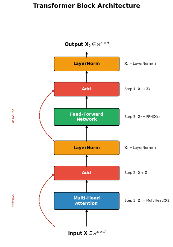
ax.set_title("Transformer Block Architecture", fontsize=14, fontweight="bold", pad=12)

cx = 1.5   # center x for main blocks
bw = 3.0   # block width

# Input
ax.text(cx + bw/2, 0.0, r"Input $\mathbf{X} \in \mathbb{R}^{n \times d}$",
        ha="center", va="center", fontsize=11, fontweight="bold")

# Multi-Head Attention
y_mha = 1.2
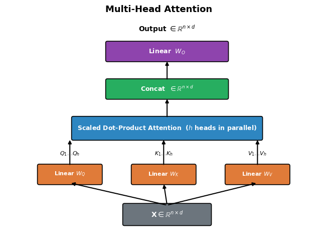
draw_box(ax, (cx, y_mha), bw, 0.7, "Multi-Head\nAttention", color="#2E86C1", fontsize=10)
draw_arrow(ax, (cx + bw/2, 0.3), (cx + bw/2, y_mha))

# Add (residual)
y_add1 = 2.6
draw_box(ax, (cx, y_add1), bw, 0.55, "Add", color="#E74C3C", fontsize=10)
draw_arrow(ax, (cx + bw/2, y_mha + 0.7), (cx + bw/2, y_add1))
# Residual arrow
draw_curved_arrow(ax, (cx, 0.3), (cx, y_add1 + 0.275), connectionstyle="arc3,rad=-0.6")
ax.text(-0.5, (0.3 + y_add1 + 0.275)/2, "residual", fontsize=8, color="#C0392B",
        ha="center", va="center", rotation=90, style="italic")

# LayerNorm 1
y_ln1 = 3.8
draw_box(ax, (cx, y_ln1), bw, 0.55, "LayerNorm", color="#F39C12", fontsize=10, text_color="black")
draw_arrow(ax, (cx + bw/2, y_add1 + 0.55), (cx + bw/2, y_ln1))

# FFN
y_ffn = 5.2
draw_box(ax, (cx, y_ffn), bw, 0.7, "Feed-Forward\nNetwork", color="#27AE60", fontsize=10)
draw_arrow(ax, (cx + bw/2, y_ln1 + 0.55), (cx + bw/2, y_ffn))

# Add (residual) 2
y_add2 = 6.6
draw_box(ax, (cx, y_add2), bw, 0.55, "Add", color="#E74C3C", fontsize=10)
draw_arrow(ax, (cx + bw/2, y_ffn + 0.7), (cx + bw/2, y_add2))
# Residual arrow
draw_curved_arrow(ax, (cx, y_ln1 + 0.55), (cx, y_add2 + 0.275), connectionstyle="arc3,rad=-0.6")
ax.text(-0.5, (y_ln1 + 0.55 + y_add2 + 0.275)/2, "residual", fontsize=8, color="#C0392B",
        ha="center", va="center", rotation=90, style="italic")

# LayerNorm 2
y_ln2 = 7.8
draw_box(ax, (cx, y_ln2), bw, 0.55, "LayerNorm", color="#F39C12", fontsize=10, text_color="black")
draw_arrow(ax, (cx + bw/2, y_add2 + 0.55), (cx + bw/2, y_ln2))

# Output
ax.text(cx + bw/2, 9.0, r"Output $\mathbf{X}_2 \in \mathbb{R}^{n \times d}$",
        ha="center", va="center", fontsize=11, fontweight="bold")
draw_arrow(ax, (cx + bw/2, y_ln2 + 0.55), (cx + bw/2, 8.7))

# Step labels on the right
annotations = [
    (y_mha + 0.35, "Step 1: $\\mathbf{Z}_1 = \\mathrm{MultiHead}(\\mathbf{X})$"),
    (y_add1 + 0.275, "Step 2: $\\mathbf{X} + \\mathbf{Z}_1$"),
    (y_ln1 + 0.275, "$\\mathbf{X}_1 = \\mathrm{LayerNorm}(\\cdot)$"),
    (y_ffn + 0.35, "Step 3: $\\mathbf{Z}_2 = \\mathrm{FFN}(\\mathbf{X}_1)$"),
    (y_add2 + 0.275, "Step 4: $\\mathbf{X}_1 + \\mathbf{Z}_2$"),
    (y_ln2 + 0.275, "$\\mathbf{X}_2 = \\mathrm{LayerNorm}(\\cdot)$"),
]
for y, txt in annotations:
    ax.text(cx + bw + 0.3, y, txt, fontsize=8, va="center", color="#333")

fig.tight_layout()
plt.show()

7.4 Second Add and Norm

\[ \mathbf{X}_2 = \operatorname{LayerNorm}(\mathbf{X}_1 + \mathbf{Z}_2). \]

The output shape is preserved: \(\mathbb{R}^{n \times d}\).

NoneAlgorithm

Full Transformer Block

Input: \(\mathbf{X} \in \mathbb{R}^{n \times d}\)

  1. Multi-head attention: \(\mathbf{Z}_1 = \operatorname{MultiHead}(\mathbf{X})\)
  2. Add and norm: \(\mathbf{X}_1 = \operatorname{LayerNorm}(\mathbf{X} + \mathbf{Z}_1)\)
  3. Feed-forward: \(\mathbf{Z}_2 = \operatorname{FFN}(\mathbf{X}_1)\)
  4. Add and norm: \(\mathbf{X}_2 = \operatorname{LayerNorm}(\mathbf{X}_1 + \mathbf{Z}_2)\)

Output: \(\mathbf{X}_2 \in \mathbb{R}^{n \times d}\)

The critical property is that the output dimension matches the input dimension, enabling stacking.

Show code
import matplotlib.pyplot as plt
import matplotlib.patches as mpatches

def draw_box(ax, xy, w, h, text, color="#4A90D9", fontsize=9, text_color="white"):
    rect = mpatches.FancyBboxPatch(xy, w, h, boxstyle="round,pad=0.06",
                                    facecolor=color, edgecolor="black", linewidth=1.2)
    ax.add_patch(rect)
    ax.text(xy[0] + w/2, xy[1] + h/2, text, ha="center", va="center",
            fontsize=fontsize, fontweight="bold", color=text_color)

def draw_arrow(ax, start, end):
    ax.annotate("", xy=end, xytext=start,
                arrowprops=dict(arrowstyle="-|>", color="black", lw=1.5))

# --- Stacked Transformer Model Diagram ---
fig, ax = plt.subplots(figsize=(6, 9))
ax.set_xlim(-1, 7)
ax.set_ylim(-0.5, 12)
ax.set_aspect("equal")
ax.axis("off")
ax.set_title("Stacked Transformer Model", fontsize=14, fontweight="bold", pad=12)

cx = 1.5
bw = 3.0

# Token input
ax.text(cx + bw/2, 0.0, r"Token IDs  $\in \mathbb{N}^n$",
        ha="center", va="center", fontsize=10, fontweight="bold")

# Token embedding
y = 1.0
draw_box(ax, (cx, y), bw, 0.6, "Token Embedding", color="#6C757D", fontsize=9)
draw_arrow(ax, (cx + bw/2, 0.3), (cx + bw/2, y))

# Positional embedding (side)
draw_box(ax, (cx + bw + 0.5, y), 2.0, 0.6, "Positional\nEncoding", color="#6C757D", fontsize=8)
ax.annotate("", xy=(cx + bw, y + 0.3), xytext=(cx + bw + 0.5, y + 0.3),
            arrowprops=dict(arrowstyle="-|>", color="black", lw=1.2))
ax.text(cx + bw + 0.25, y + 0.55, "+", fontsize=14, fontweight="bold", ha="center")

# X^(0)
y_x0 = 2.2
ax.text(cx + bw/2, y_x0, r"$\mathbf{X}^{(0)} \in \mathbb{R}^{n \times d}$",
        ha="center", va="center", fontsize=10)
draw_arrow(ax, (cx + bw/2, y + 0.6), (cx + bw/2, y_x0 - 0.2))

# Transformer blocks
block_colors = ["#2E86C1", "#2980B9", "#2471A3", "#1F618D"]
L = 4
y_start = 3.0
block_h = 0.7
gap = 1.1
for i in range(L):
    yb = y_start + i * gap
    if i < 3:
        label = f"Transformer Block {i+1}"
        draw_box(ax, (cx, yb), bw, block_h, label,
                 color=block_colors[i], fontsize=9)
    else:
        # Ellipsis then final block
        y_dots = y_start + 2 * gap + block_h + 0.15
        ax.text(cx + bw/2, y_dots + 0.15, "⋮", ha="center", va="center", fontsize=20, color="#555")
        yb_final = y_dots + 0.7
        draw_box(ax, (cx, yb_final), bw, block_h, f"Transformer Block $L$",
                 color=block_colors[3], fontsize=9)

    # Arrows between blocks
    if i == 0:
        draw_arrow(ax, (cx + bw/2, y_x0 + 0.2), (cx + bw/2, yb))
    elif i < 3:
        draw_arrow(ax, (cx + bw/2, y_start + (i-1)*gap + block_h),
                   (cx + bw/2, yb))

# Arrow from block 2 to dots
draw_arrow(ax, (cx + bw/2, y_start + 2*gap + block_h),
           (cx + bw/2, y_start + 2*gap + block_h + 0.15))
# Arrow from dots to block L
y_dots = y_start + 2 * gap + block_h + 0.15
yb_final = y_dots + 0.7
draw_arrow(ax, (cx + bw/2, y_dots + 0.4), (cx + bw/2, yb_final))

# Shape annotations on the right
for i in range(3):
    yb = y_start + i * gap + block_h / 2
    ax.text(cx + bw + 0.3, yb, r"$\mathbb{R}^{n \times d}$", fontsize=9, va="center", color="#555")
ax.text(cx + bw + 0.3, yb_final + block_h/2, r"$\mathbb{R}^{n \times d}$",
        fontsize=9, va="center", color="#555")

# Output head
y_head = yb_final + block_h + 0.8
draw_box(ax, (cx, y_head), bw, 0.6, "Linear Output Head", color="#8E44AD", fontsize=9)
draw_arrow(ax, (cx + bw/2, yb_final + block_h), (cx + bw/2, y_head))

# Logits
ax.text(cx + bw/2, y_head + 1.0,
        r"Logits $\in \mathbb{R}^{n \times |\mathcal{V}|}$",
        ha="center", va="center", fontsize=10, fontweight="bold")
draw_arrow(ax, (cx + bw/2, y_head + 0.6), (cx + bw/2, y_head + 0.75))

fig.tight_layout()
plt.show()

import torch
import torch.nn as nn

class TransformerBlock(nn.Module):
    """
    A single transformer block: MultiHeadAttention + FFN,
    each with residual connection and layer normalization.
    """
    def __init__(self, d_model, num_heads, d_ff):
        super().__init__()
        self.attn = MultiHeadAttention(d_model, num_heads)
        self.norm1 = nn.LayerNorm(d_model)
        self.ffn = nn.Sequential(
            nn.Linear(d_model, d_ff),
            nn.ReLU(),
            nn.Linear(d_ff, d_model),
        )
        self.norm2 = nn.LayerNorm(d_model)

    def forward(self, X, mask=None):
        # Sub-layer 1: Multi-head attention + add & norm
        Z1 = self.attn(X, mask=mask)
        X1 = self.norm1(X + Z1)

        # Sub-layer 2: FFN + add & norm
        Z2 = self.ffn(X1)
        X2 = self.norm2(X1 + Z2)

        return X2


# --- Verify shape preservation ---
d_model, num_heads, d_ff, seq_len = 64, 8, 256, 10
block = TransformerBlock(d_model, num_heads, d_ff)
X = torch.randn(seq_len, d_model)
output = block(X)
print(f"Input shape:  {X.shape}")      # (10, 64)
print(f"Output shape: {output.shape}")  # (10, 64)

Part 8 — Stacking Transformer Blocks

A deep transformer model is built by stacking \(L\) identical transformer blocks. Let \(L\) be the number of layers.

The initial representation is formed by combining token and positional embeddings:

\[ \mathbf{X}^{(0)} = \mathbf{E}_{\text{token}} + \mathbf{E}_{\text{pos}}. \]

For \(\ell = 1, \dots, L\):

\[ \mathbf{X}^{(\ell)} = \operatorname{TransformerBlock} \left( \mathbf{X}^{(\ell-1)} \right). \]

The final representation \(\mathbf{X}^{(L)} \in \mathbb{R}^{n \times d}\) is then passed to a task-specific head (e.g., a linear layer mapping to vocabulary logits).

import torch
import torch.nn as nn

class SimpleTransformer(nn.Module):
    """
    A simple transformer model: token embedding + positional embedding
    + L stacked transformer blocks + linear output head.
    """
    def __init__(self, vocab_size, d_model, num_heads, d_ff, num_layers, max_seq_len):
        super().__init__()
        self.token_emb = nn.Embedding(vocab_size, d_model)
        self.pos_emb = nn.Embedding(max_seq_len, d_model)
        self.blocks = nn.ModuleList([
            TransformerBlock(d_model, num_heads, d_ff)
            for _ in range(num_layers)
        ])
        self.output_head = nn.Linear(d_model, vocab_size)

    def forward(self, tokens, mask=None):
        n = tokens.shape[0]
        positions = torch.arange(n, device=tokens.device)

        # Combine token and positional embeddings
        X = self.token_emb(tokens) + self.pos_emb(positions)

        # Pass through L transformer blocks
        for block in self.blocks:
            X = block(X, mask=mask)

        # Project to vocabulary logits
        logits = self.output_head(X)
        return logits


# --- Example: small autoregressive transformer ---
vocab_size = 1000
d_model, num_heads, d_ff = 64, 8, 256
num_layers, max_seq_len = 4, 128

model = SimpleTransformer(vocab_size, d_model, num_heads, d_ff, num_layers, max_seq_len)
tokens = torch.randint(0, vocab_size, (20,))  # sequence of 20 tokens

# Create causal mask
n = tokens.shape[0]
causal_mask = torch.triu(torch.full((n, n), float('-inf')), diagonal=1)

logits = model(tokens, mask=causal_mask)
print(f"Token input shape: {tokens.shape}")   # (20,)
print(f"Logit output shape: {logits.shape}")   # (20, 1000)

Part 9 — Why Transformers as Universal Backbone

The transformer has become the dominant architecture not just for language modeling, but across many domains including vision, speech, and multimodal learning. Several properties make it an exceptionally effective universal backbone:

  • Model arbitrary pairwise token interactions. The attention mechanism allows any token to attend to any other token, enabling the model to capture dependencies regardless of distance.
  • Provide global receptive field at every layer. Unlike convolutions (which have a fixed local receptive field) or RNNs (which must propagate information sequentially), every transformer layer has access to the entire input.
  • Enable parallel computation. All positions are processed simultaneously, leading to efficient utilization of modern GPU and TPU hardware.
  • Preserve representation dimension \(d\). The shape invariance across layers (\(\mathbb{R}^{n \times d} \to \mathbb{R}^{n \times d}\)) makes the architecture modular and easy to scale.
  • Scale naturally with depth \(L\). Adding more layers simply stacks more identical blocks, and empirical evidence shows consistent improvement with depth (given sufficient data and compute).

Conclusion

In this lesson, we have built the transformer architecture from the ground up:

  1. We formalized the tensor shapes for autoregressive, masked, and sequence-to-sequence language modeling.
  2. We defined the attention operator as a weighted aggregation and specialized it to scaled dot-product attention.
  3. We introduced the causal mask for enforcing autoregressive constraints.
  4. We extended single-head attention to multi-head attention, showing how it enables diverse attention patterns.
  5. We distinguished self-attention from cross-attention.
  6. We explained why positional encoding is necessary and how it is injected.
  7. We assembled the full transformer block from attention, residual connections, layer normalization, and a feed-forward network.
  8. We showed how blocks are stacked to form deep models.

These components form the foundation of modern language models such as GPT, BERT, and T5, and understanding them is essential for working with any transformer-based system.